0050.XGB.180D. 1'st.practice

2024-06-19

!pip install yfinance

import yfinance as yf

# 下載0050過去5年的股價數據
ticker = '0050.TW'
stock_data = yf.download(ticker, period='5y')
stock_data.reset_index(inplace=True)
stock_data.to_csv('0050_stock_data.csv', index=False)

import pandas as pd
import numpy as np
import matplotlib.pyplot as plt
from sklearn.preprocessing import MinMaxScaler
import tensorflow as tf
from tensorflow.keras.models import Sequential
from tensorflow.keras.layers import Dense, LSTM
from sklearn.metrics import mean_squared_error
import math

# 加載數據
df = pd.read_csv('0050_stock_data.csv')
df = df[['Date', 'Close']]

# 數據歸一化
scaler = MinMaxScaler(feature_range=(0, 1))
df_scaled = scaler.fit_transform(df[['Close']])

# 創建訓練和測試集
train_size = int(len(df_scaled) * 0.8)
test_size = len(df_scaled) - train_size
train_data, test_data = df_scaled[0:train_size, :], df_scaled[train_size:len(df_scaled), :]

# 創建數據集
def create_dataset(dataset, time_step=1):
    dataX, dataY = [], []
    for i in range(len(dataset) - time_step - 1):
        a = dataset[i:(i + time_step), 0]
        dataX.append(a)
        dataY.append(dataset[i + time_step, 0])
    return np.array(dataX), np.array(dataY)

time_step = 100
X_train, Y_train = create_dataset(train_data, time_step)
X_test, Y_test = create_dataset(test_data, time_step)

# 調整數據格式以適應LSTM輸入
X_train = X_train.reshape(X_train.shape[0], X_train.shape[1], 1)
X_test = X_test.reshape(X_test.shape[0], X_test.shape[1], 1)

# 構建LSTM模型
model = Sequential()
model.add(LSTM(50, return_sequences=True, input_shape=(time_step, 1)))
model.add(LSTM(50, return_sequences=False))
model.add(Dense(25))
model.add(Dense(1))

# 編譯模型
model.compile(optimizer='adam', loss='mean_squared_error')

# 訓練模型
model.fit(X_train, Y_train, batch_size=1, epochs=10)

import matplotlib.dates as mdates

# 確保日期列的格式正確
df['Date'] = pd.to_datetime(df['Date'])

# 預測數據
train_predict = model.predict(X_train)
test_predict = model.predict(X_test)

# 反歸一化預測結果
train_predict = scaler.inverse_transform(train_predict)
test_predict = scaler.inverse_transform(test_predict)
Y_train = scaler.inverse_transform(np.array(Y_train).reshape(-1, 1))
Y_test = scaler.inverse_transform(np.array(Y_test).reshape(-1, 1))

# 計算RMSE
train_rmse = math.sqrt(mean_squared_error(Y_train, train_predict))
test_rmse = math.sqrt(mean_squared_error(Y_test, test_predict))
print(f'Train RMSE: {train_rmse}')
print(f'Test RMSE: {test_rmse}')

# 繪製訓練數據的預測結果
train_predict_plot = np.empty_like(df_scaled)
train_predict_plot[:, :] = np.nan
train_predict_plot[time_step:len(train_predict) + time_step, :] = train_predict

# 繪製測試數據的預測結果
test_predict_plot = np.empty_like(df_scaled)
test_predict_plot[:, :] = np.nan
test_predict_plot[len(train_predict) + (time_step * 2) + 1:len(df_scaled) - 1, :] = test_predict

# 預測未來180天
future_days = 180
temp_input = list(test_data[-time_step:].flatten())

# 確保 temp_input 的長度正確
assert len(temp_input) == time_step, f"temp_input 的長度不正確：{len(temp_input)}，應該是 {time_step}"

# 迭代預測未來的數據
future_predictions = []
for i in range(future_days):
    if len(temp_input) > time_step:
        temp_input = temp_input[-time_step:]
    try:
        input_data = np.array(temp_input).reshape((1, time_step, 1))
    except ValueError as e:
        print(f"Error at iteration {i}: {e}")
        print(f"temp_input: {temp_input}")
        break
    future_prediction = model.predict(input_data)
    temp_input.append(future_prediction[0][0])
    future_predictions.append(future_prediction[0][0])

# 反歸一化未來預測結果
if len(future_predictions) > 0:  # 確保有未來的預測結果
    future_predictions = scaler.inverse_transform(np.array(future_predictions).reshape(-1, 1))

    # 繪製結果
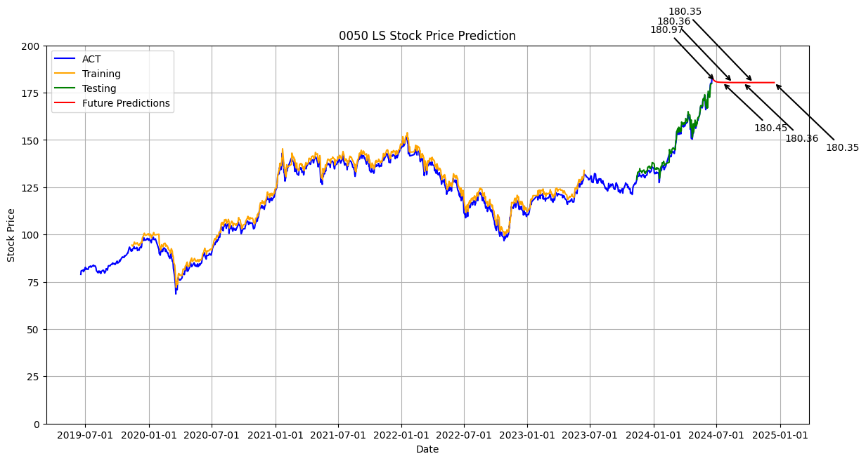
    plt.figure(figsize=(14, 7))
    plt.plot(df['Date'], scaler.inverse_transform(df_scaled), label='ACT', color='blue')
    plt.plot(df['Date'], train_predict_plot, label='Training', color='orange')
    plt.plot(df['Date'], test_predict_plot, label='Testing', color='green')

    # 繪製未來180天的預測結果
    future_dates = pd.date_range(start=df['Date'].iloc[-1], periods=future_days + 1).tolist()
    plt.plot(future_dates[1:], future_predictions, label='Future Predictions', color='red')

    # 標示特定日期的收盤價
    specific_days = [10, 30, 60, 90, 120, 180]
    offsets = [(-50, 50), (50, -50), (-60, 60), (60, -60), (-70, 70), (70, -70)]  # 进一步增加间距
    for i, day in enumerate(specific_days):
        plt.annotate(f'{future_predictions[day-1][0]:.2f}',
                     (future_dates[day], future_predictions[day-1]),
                     textcoords="offset points",
                     xytext=offsets[i],
                     ha='center',
                     arrowprops=dict(arrowstyle='->', lw=1.5, color='black'),
                     color='black')

    # 設置 x 軸標記為每半年
    ax = plt.gca()
    ax.xaxis.set_major_locator(mdates.MonthLocator(bymonth=[1, 7], bymonthday=1))
    ax.xaxis.set_major_formatter(mdates.DateFormatter('%Y-%m-%d'))

    # 設置 y 軸範圍
    plt.ylim(0, 200)

    plt.xlabel('Date')
    plt.ylabel('Stock Price')
    plt.title('0050 LS Stock Price Prediction')
    plt.legend(loc='upper left')
    plt.grid(True)
    plt.show()
else:
    print("No future predictions to plot.")