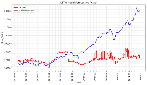
Predict TAIEX.s46_LSTM(3). Future select by Forest 使用決策樹回歸進行特徵選擇,並使用選擇的特徵來訓練 LSTM 模型。最後打印所選的特徵變數並顯示實際值和預測值的圖表。 import os import pandas as pd import numpy as np import matplotlib.pyplot as plt import matplotlib.dates as mdates from sklearn.metrics import mean_squared_error, mean_absolute_error from sklearn.preprocessing import MinMaxScaler from sklearn.ensemble import RandomForestRegressor from tensorflow.keras.models import
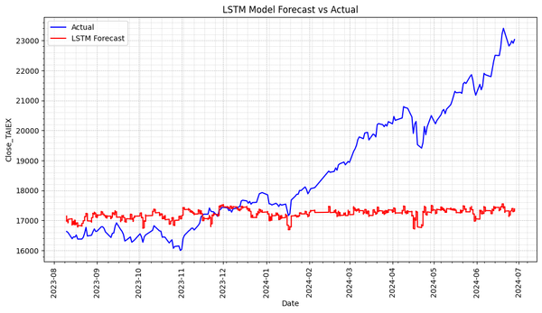
Predict TAIEX.s46_LSTM(2). Future select by Decision Tree. 使用決策樹進行特徵選擇,並使用選擇的特徵來訓練 LSTM 模型。 最後打印所選的特徵變數並顯示實際值和預測值圖 import os import pandas as pd import numpy as np import matplotlib.pyplot as plt import matplotlib.dates as mdates from sklearn.metrics import mean_squared_error, mean_absolute_error from sklearn.preprocessing import MinMaxScaler from sklearn.tree import DecisionTreeRegressor from tensorflow.keras.models import
Predict TAIEX.s45_LSTM. Adj_Close 1. 特徵工程:使用 Adj_Close 計算移動平均線(MA7 和 MA21)、RSI 和 MACD。 2. 特徵選擇:使用隨機森林模型選擇最重要的特徵。 3. 數據標準化:將特徵和目標變量標準化。 4. 創建序列:為 LSTM 模型創建時間序列數據。 5. 構建 LSTM 模型:使用選擇的特徵來訓練 LSTM 模型。 6. 預測和評估:進行預測並計算誤差(MSE 和 MAE)。 7. 可視化:繪製實際值和預測值的圖表。 8. 打印特徵變數:打印所選的特徵變數。 source code import os import pandas as pd
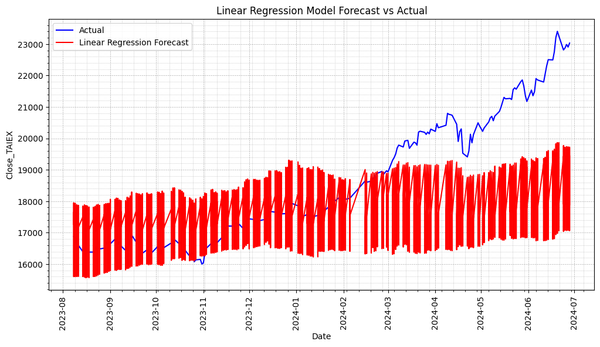
Predict **TAIEX.s44_Linear Regression. import os import pandas as pd import numpy as np import matplotlib.pyplot as plt import matplotlib.dates as mdates from sklearn.metrics import mean_squared_error, mean_absolute_error from sklearn.feature_selection import SelectKBest, f_regression from sklearn.linear_model import LinearRegression from sklearn.model_selection import train_
Essay 希望.0703 寫給今新到來的新員工 Verse 1 在那微光初現的清晨 新生命的哭聲劃破寧靜 媽媽的眼中閃爍著淚光 那是愛和希望的交織 Chorus 希望在你的手心中跳動 每一次擁抱都是愛的傳遞 你的世界因你而美麗 新生命我們一同迎接奇蹟 Verse 2 小小的手握住了未來 每一步都是新的探索 媽媽的心中充滿著期盼 願你的人生充滿著光彩 Chorus 希望在你的手心中跳動 每一次擁抱都是愛的傳遞 你的世界因你而美麗 新生命我們一同迎接奇蹟 Bridge 無論前方多麼遙遠 媽媽會在你身旁守候 你的笑容是我最大的財寶 陪你走過每一段旅途 Chorus 希望在你的手心中跳動 每一次擁抱都是愛的傳遞 你的世界因你而美麗 新生命我們一同迎接奇蹟 Outro 在這充滿希望的未來 媽媽的愛永遠不變 新生命願你永遠幸福 這首希望的歌永遠為你而唱
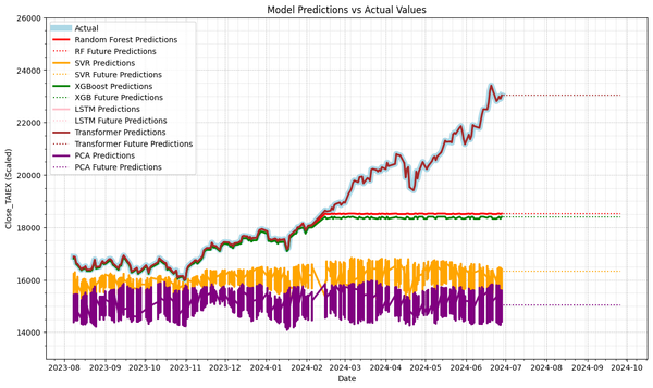
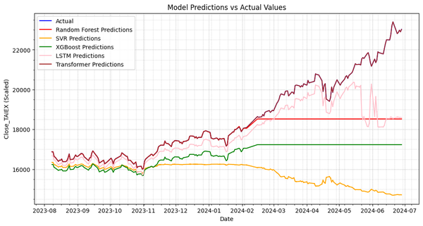
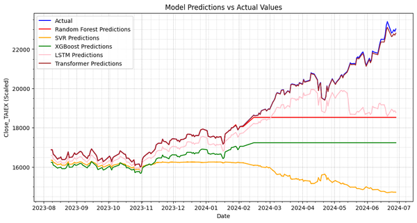
Predict TAIEX.s92_使用 RandomForest 選擇特徵值,增加 Future Prediction Line 1. Transformer Prediction 有可能存在過擬合問題 2. Future Prediction Line 未 Training Output Index(['Date', 'ST_Code', 'ST_Name', 'Open', 'High', 'Low', 'Close', 'Adj_Close', 'Volume', 'MA7', 'MA21', 'MA50&
Predict TAIEX.s91_練習使用 RandomForest 選擇特徵值的用法 + RFE 試作 Output Shapes: test_labels: (6540,) transformer_predictions: (6540, 10) Adjusted transformer_predictions shape: (6540,) Random Forest MSE: 2545495.9702350823 SVR MSE: 9719829.364170404 XGBoost MSE: 2829341.20223588 LSTM MSE: 346273600.6513799 Transformer MSE: 16777426.64694445 Random Forest MAE: 903.3660629908254 SVR MAE: 2474.4028472217 XGBoost MAE: 999.7728105920297 LSTM MAE:
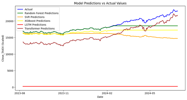
Predict **TAIEX.s43_Training.3th.RandomForest+SVR+XGB+Transformer. 訓練4 Picture 1 Shapes: test_labels: (6540,) transformer_predictions: (6540, 2) Adjusted transformer_predictions shape: (6540,) Random Forest MSE: 2538928.7593811294 SVR MSE: 13866232.38063333 XGBoost MSE: 5859048.980611635 LSTM MSE: 1862506.720476739 Transformer MSE: 0.020672246942703427 import os import pandas as pd import numpy as np import matplotlib.pyplot as
Predict **TAIEX.s43_Training.3th.RandomForest+SVR+XGB+Transformer. 訓練3 transformer_predictions: (6540, 2) Adjusted transformer_predictions shape: (6540,) Random Forest MSE: 2539254.211486759 SVR MSE: 13866232.398817357 XGBoost MSE: 5859048.979625798 LSTM MSE: 1753263.4853189574 Transformer MSE: 2732.7598143748187 import os import pandas as pd import numpy as np import matplotlib.pyplot as plt import matplotlib.dates as mdates
Predict **TAIEX.s42_Training.2nd.RandomForest+SVR+XGB+Transformer. 簡易訓練 import os import pandas as pd import numpy as np import matplotlib.pyplot as plt import matplotlib.dates as mdates from sklearn.preprocessing import StandardScaler from sklearn.ensemble import RandomForestRegressor from sklearn.svm import SVR import tensorflow as tf from tensorflow.keras.models import Sequential from tensorflow.keras.layers import
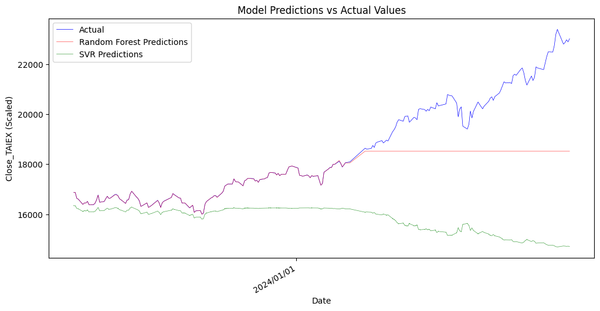
Predict TAIEX.s41_Training.1'st.第一次訓練,RandomForest+SVR import pandas as pd import numpy as np import matplotlib.pyplot as plt import matplotlib.dates as mdates from sklearn.preprocessing import StandardScaler from sklearn.ensemble import RandomForestRegressor from sklearn.svm import SVR # 加載數據 file_path = '/content/drive/My Drive/MSCI_Taiwan_30_data_with_OBV.csv' data
Predict **TAIEX.s30_Future_Engineering.特徵工程 import pandas as pd import numpy as np from sklearn.preprocessing import StandardScaler # 加載數據 file_path = '/content/drive/My Drive/MSCI_Taiwan_30_data_with_OBV.csv' data = pd.read_csv(file_path) # 更改列名 data.rename(columns={'Close_MSCI': 'Close'}, inplace=True) # 1. 計算移動平均線
Predict **TAIEX.ML.s20_Missing Values Analysis.缺失值分析(填補重製) # Missing values analysis missing_values = data.isnull().sum() print("Missing Values Analysis:") print(missing_values) Missing Values Analysis: Date 0 ST_Code 0 ST_Name 0 Open 0 High 0 Low 0 Close_MSCI 0 Adj_Close 0 Volume 0 MA7 180 MA21 600 MA50 1470 MA100 2970
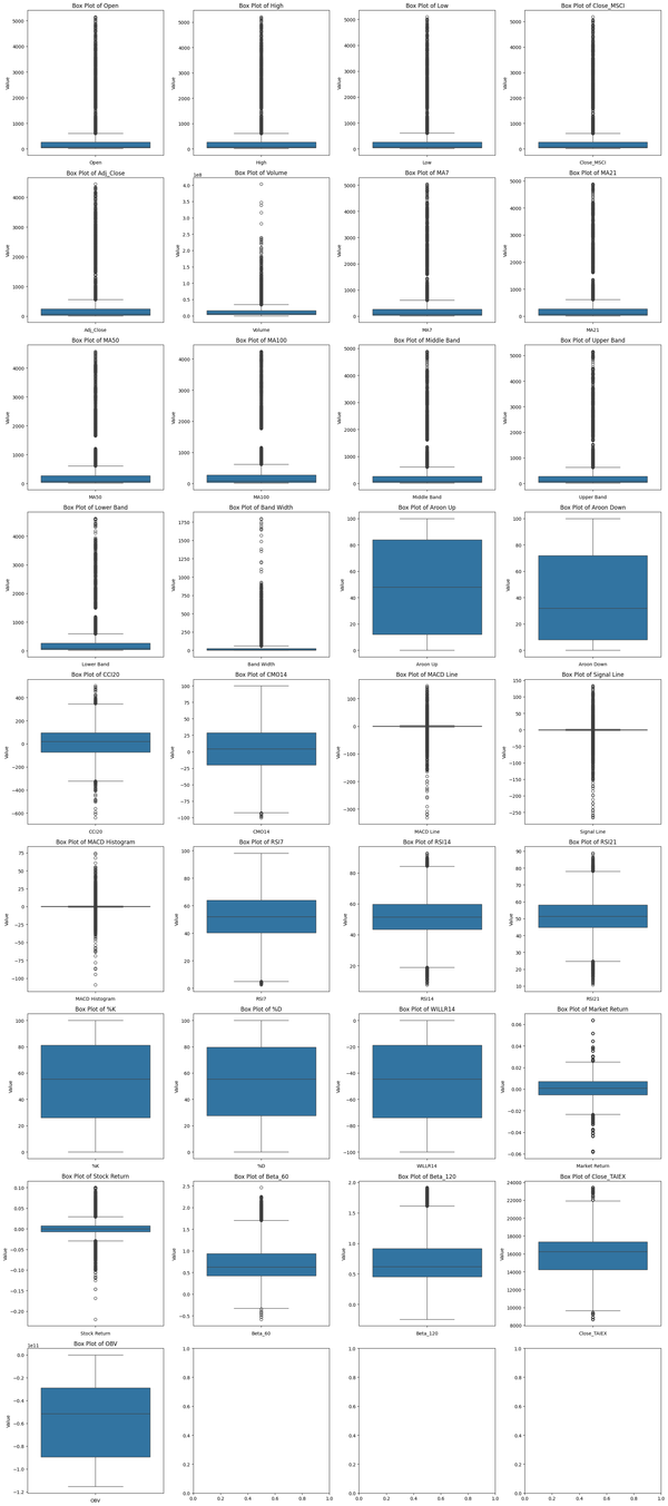
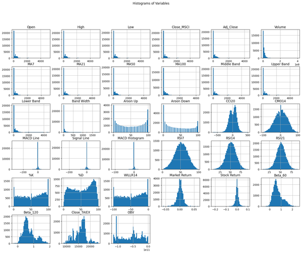
Predict **TAIEX.ML.s14_Box Plot.箱型圖 Box Plot Matrix Map 提供了對各變數數據分佈的直觀了解,有助於識別數據中的異常值和分佈特徵。通過觀察這些圖表,可以為後續的數據清洗和特徵工程提供參考。 Box Plot Matrix Map 圖表顯示了每個變數的數據分佈情況,其中包括中位數、四分位數範圍、異常值等信息。以下是圖表的摘要說明: 1. 數據範圍: * 大多數變數的數據範圍較小,集中在較低的數值區間。 * Volume 和 OBV 的數據範圍明顯大於其他變數,因此在圖表中顯示時有較大的差異。 2. 異常值(Outliers): * 幾乎所有變數都存在異常值,這些異常值顯示為圖表中的小圓點。 * 特別是 Volume、Band Width、MACD Line、Signal Line 等變數,異常值較多且分佈較廣。 3. 變數分佈: * 部分變數(如 Aroon Up、Aroon Down、RSI7、
Predict **TAIEX.ML.s13_Normality_Test.常態分配檢定 正常性檢驗結果顯示所有變數的 p 值均為 0,表明數據顯著偏離正態分佈。 這是正常的結果,因為股票市場數據通常不遵循正態分佈。 * P 值 (p-value):在統計檢驗中,P 值用於衡量觀察結果與零假設(通常是數據符合某種分佈,比如正態分佈)的偏離程度。當 P 值小於某個顯著性水平(如 0.05)時,我們通常拒絕零假設。 * 正常性檢驗:常見的正態性檢驗方法包括 Shapiro-Wilk 檢驗。在這種檢驗中,零假設是數據來自正態分佈。 在我們的檢驗中,所有變數的 P 值均為 0(或極小),這意味著我們有足夠的證據拒絕數據來自正態分佈的假設。這在股票市場數據中是正常現象,因為這些數據往往具有尖峰厚尾(leptokurtic)或偏態(skewness),不符合正態分佈。 # Sample data sampled_data = data.sample(n=
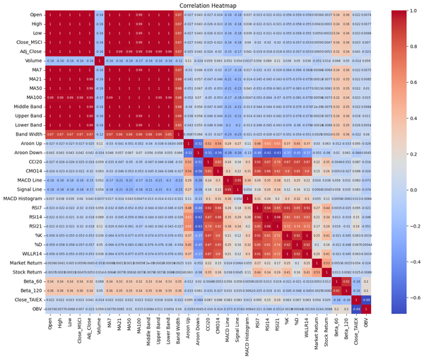
Predict **TAIEX.ML.s12_Correlation Heatmap.熱點圖(1) # Select only numeric columns for correlation analysis numeric_data = data.select_dtypes(include=[float, int]) # Correlation analysis correlation_matrix = numeric_data.corr() print("Correlation Matrix:") print(correlation_matrix) # Plot correlation heatmap plt.figure(figsize=(16, 12)) sns.heatmap(correlation_matrix, annot=True, cmap='coolwarm') plt.title(
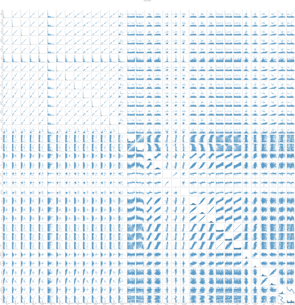
Predict **TAIEX.ML.s11_Scatter Plot.散布圖(2) # Sample data sampled_data = data.sample(n=1000, random_state=42) # Plot pairwise relationships sns.pairplot(sampled_data) plt.suptitle('Scatter Plot of Variables', y=1.02) plt.show()
Predict **TAIEX.ML.s11_Scatter Plot.散布圖(1) '**有些變數的視覺化趨勢就蠻明顯的(見下圖) import pandas as pd import numpy as np import matplotlib.pyplot as plt import seaborn as sns from scipy.stats import pearsonr # Mount Google Drive from google.colab import drive drive.mount('/content/drive', force_remount=True) # Load the data file_path = '/content/drive/
Predict TAIEX.ML.s02_Dataset.數據描述 from google.colab import drive drive.mount('/content/drive') import pandas as pd import matplotlib.pyplot as plt import seaborn as sns from scipy import stats # Load the data file_path = '/content/drive/My Drive/MSCI_Taiwan_30_data_with_OBV.csv' data = pd.read_csv(
Predict TAIEX.ML.s01_Varians.變數說明 變數名稱 說明 Close_TAIEX TAIEX 指數的收盤價 Adj_Close 收盤價 Aroon Down Aroon 指標中的下降線 Aroon Up Aroon 指標中的上升線 Band Width 布林帶的寬度 Beta_120 過去 120 天的 Beta 值 Beta_60 過去 60 天的 Beta 值 CCI20 20 天商品通道指數 Close 收盤價 CMO14 14 天的錢德動量震盪指標 %D 隨機指標中的 %D 線 Date 日期 High 最高價
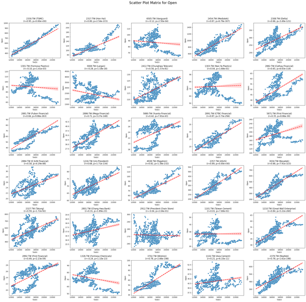
Predict **Scatter Matrix by Varians and ST_Stock ( P<0.05) Mounted at /content/drive Overall Pearson Correlation with Close_TAIEX: Pearson Correlation P-value RSI21 0.185104 2.388407e-245 RSI14 0.151384 6.581929e-165 CMO14 0.098249 4.022700e-70 Aroon Up 0.095180 3.432801e-65 RSI7 0.094756 9.565736e-66 CCI20 0.087107 3.717489e-55 Signal Line 0.083004 1.343307e-49
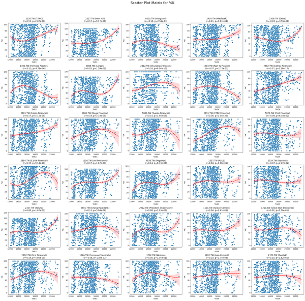
practice Scatter Matrix by ST_Stock. Pearson Correlation with Close_TAIEX for 2330.TW (TSMC) Pearson Correlation P-value Close_TAIEX_TAIEX 1.000000 0.000000e+00 Adj_Close 0.954742 0.000000e+00 Low 0.951000 0.000000e+00 MA7 0.950148 0.000000e+00 Middle Band 0.949835 0.000000e+00 MA21 0.949652 0.
practice Close_TAIEX -N.Scatter Plot Matrix_0630 import pandas as pd import numpy as np import matplotlib.pyplot as plt import seaborn as sns from scipy.stats import pearsonr # Mount Google Drive from google.colab import drive drive.mount('/content/drive', force_remount=True) # Load the data file_path = '/content/drive/My Drive/MSCI_
practice Heat MAP.MSCI 個股對 TAIEX 的 Pearson analysis.(f)0630 MSCI 個股對 TAIEX 的 Pearson analysis import pandas as pd import numpy as np import matplotlib.pyplot as plt import seaborn as sns from scipy.stats import pearsonr # Mount Google Drive from google.colab import drive drive.mount('/content/drive', force_remount=True) # Load the data file_path
MSCI.TW30.Pearson correlation coefficient,Draft,發散的亂算 import pandas as pd import numpy as np import matplotlib.pyplot as plt import seaborn as sns from scipy.stats import pearsonr # Mount Google Drive from google.colab import drive drive.mount('/content/drive', force_remount=True) # Load the data file_path = '/content/drive/My Drive/MSCI_