CPBL,Pitcher Pan's Performance, 372game


Descriptive Statistics
Pearson Correlation Analysis with H (安打)
Pearson Correlation Analysis Results with 'H' as the Dependent Variable:
       Variable   R Value   P Value
5             R  0.713628  0.000000
6            ER  0.683962  0.000000
1            FB  0.679566  0.000000
2            NP  0.590262  0.000000
30        BABIP  0.588690  0.000000
17       Strike  0.582755  0.000000
0        IP_all  0.403094  0.000000
32          H/9  0.377150  0.000000
27         WHIP  0.327426  0.000000
11           FO  0.314922  0.000000
10           GO  0.304367  0.000000
3            HR  0.250577  0.000001
22  Assist_Down  0.214961  0.000029
31         BB/9  0.174454  0.000726
7            BB  0.174454  0.000726
28         P/IP  0.164857  0.001440
12    ERA_Delta  0.156666  0.002444
19   Wild_Pitch  0.114705  0.026952
21     Run_Down  0.112901  0.029467
9           HBP  0.108968  0.035651
4            SO  0.102986  0.047153
26    Check_Out  0.097535  0.060200
15          NBB  0.084153  0.105126
23  Double_Play  0.073951  0.154600
25            E  0.060870  0.241534
20        Fault  0.044601  0.391020
29        GO/AO  0.033313  0.528091
13           CG  0.016750  0.747455
33          K/9 -0.007242  0.889438
14          SHO -0.081492  0.116630
8           IBB -0.108560  0.036351
16           BS -0.113268  0.028939
18           SB       NaN       NaN
24  Triple_Play       NaN       NaN
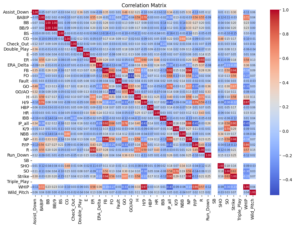
Correlation Matrix Heat map
相關矩陣圖顯示了各變數之間的Pearson相關係數。紅色表示正相關,藍色表示負相關,顏色越深,相關性越強。圖中顯示,被安打數(H)與四壞球(BB)呈現中等正相關(R = 0.58),與全壘打(HR)呈現弱正相關(R = 0.21)。投球局數(IP_all)與被安打數(H)呈現弱負相關(R = -0.21)。每九局三振數(K/9)與三振數(SO)高度正相關(R = 0.99),與防禦率變化(ERA_Delta)呈現較弱負相關(R = -0.20)。防禦率變化(ERA_Delta)與自責分(ER)高度正相關(R = 0.93),與每九局被安打數(H/9)呈現中等正相關(R = 0.55)。這些結果有助於理解投手績效的影響因素。
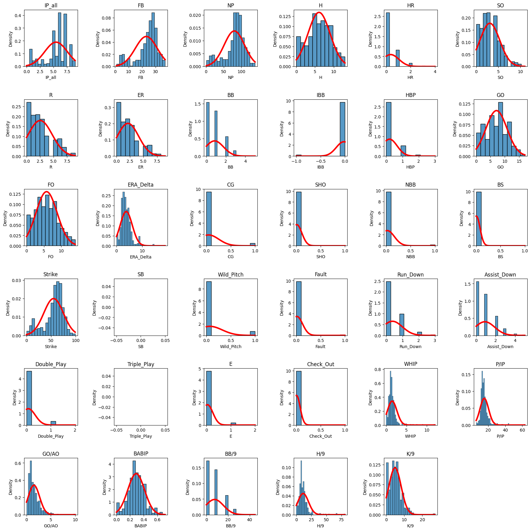
Histogram of all variables
Source Code
import pandas as pd
import numpy as np
import matplotlib.pyplot as plt
import seaborn as sns
from scipy.stats import pearsonr
# 挂载Google Drive
from google.colab import drive
drive.mount('/content/drive', force_remount=True)
# 读取数据
file_path = '/content/drive/My Drive/datan/Pan_372_2021_2.xlsx'
data = pd.read_excel(file_path)
# 按时间排序,并确保 Game_No 随时间递增
data = data.sort_values(by='Date')
data['Game_No'] = range(1, len(data) + 1)
# 去掉 'Date' 列,保留 'Game_No' 作为索引
numeric_data = data.drop(columns=['Date']).set_index('Game_No')
# 确认所有列为数值型
numeric_data = numeric_data.select_dtypes(include=[np.number])
# 设置 SB 和 Triple_Play 为 0 的值为空白
numeric_data['SB'] = numeric_data['SB'].replace(0, np.nan)
numeric_data['Triple_Play'] = numeric_data['Triple_Play'].replace(0, np.nan)
# 进行 Pearson 相关分析,使用 'H' 作为应变量
results = []
dependent_var = 'H'
for col in numeric_data.columns:
if col != dependent_var:
# 确保两列数据长度一致
valid_data = numeric_data[[dependent_var, col]].dropna()
if len(valid_data) >= 2: # 确保数据点数量至少为2
r, p = pearsonr(valid_data[dependent_var], valid_data[col])
results.append({'Variable': col, 'R Value': r, 'P Value': f'{p:.6f}'})
else:
results.append({'Variable': col, 'R Value': np.nan, 'P Value': np.nan})
# 将结果转换为 DataFrame 并显示
results_df = pd.DataFrame(results).sort_values(by='R Value', ascending=False)
# 显示结果表格
print("Pearson Correlation Analysis Results with 'H' as the Dependent Variable:")
print(results_df)
# 保存结果表格为 CSV 文件
results_df.to_csv('/content/drive/My Drive/datan/Pearson_Correlation_Results.csv', index=False)
# 繪製相關性矩陣,按字母順序排列變量
sorted_columns = sorted(numeric_data.columns)
sorted_data = numeric_data[sorted_columns]
correlation_matrix = sorted_data.corr()
plt.figure(figsize=(12, 8))
sns.heatmap(correlation_matrix, annot=True, cmap='coolwarm', fmt='.2f', annot_kws={"size": 6})
plt.title('Correlation Matrix')
plt.show()
# 繪製直方圖並加上常態分佈線,使其看起來更像正方形
fig, axes = plt.subplots(6, 6, figsize=(18, 18)) # 調整以使圖表更像正方形
axes = axes.flatten()
for i, col in enumerate(numeric_data.columns):
sns.histplot(numeric_data[col], kde=False, ax=axes[i], stat="density")
# 計算常態分佈
mean = numeric_data[col].mean()
std = numeric_data[col].std()
x = np.linspace(numeric_data[col].min(), numeric_data[col].max(), 100)
p = norm.pdf(x, mean, std)
axes[i].plot(x, p, 'r', linewidth=3.5)
axes[i].set_title(col)
axes[i].set_xlabel(col)
axes[i].set_ylabel('Density')
# 移除多餘的子圖
for ax in axes[len(numeric_data.columns):]:
ax.remove()
plt.tight_layout(pad=3.0) # 增加每列的列距
plt.show()
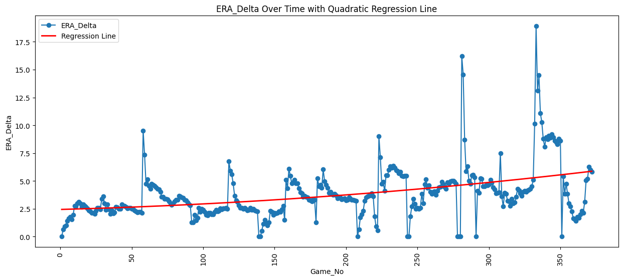
# 繪製 ERA_Delta 隨 Game_No 變化的折線圖
plt.figure(figsize=(15, 6))
plt.plot(data['Game_No'], data['ERA_Delta'], marker='o', label='ERA_Delta')
# 添加三項回歸線
p = Polynomial.fit(data['Game_No'], data['ERA_Delta'], 3)
x_new = np.linspace(data['Game_No'].min(), data['Game_No'].max(), 500)
y_new = p(x_new)
plt.plot(x_new, y_new, 'r-', label='Regression Line', linewidth=2)
plt.title('ERA_Delta Over Time with Regression Line')
plt.xlabel('Game_No')
plt.ylabel('ERA_Delta')
plt.xticks(rotation=90)
plt.legend()
plt.show()