Economic

Machine Learning | Study | K-Means 分群 | GDP Clustering

cy.lu

20 May 2024 • 5 min read

Photo by Billy Huynh / Unsplash

C.Y.LU 2024-05-20

基本概念

K-Means 的目標是將數據點分成 K 個群集，使得每個群集中的數據點彼此之間的距離最小，而與其他群集的數據點距離最大。該演算法依賴於以下幾個步驟：

選擇 K 個初始中心點（Centroids）：這些中心點可以隨機選擇，也可以使用其他方法確定。
分配數據點：將每個數據點分配給最近的中心點，形成 K 個群集。
更新中心點：重新計算每個群集的中心點，通常是該群集所有數據點的平均值。
重複步驟 2 和 3：直到中心點不再變化或達到預定的迭代次數。

演算法步驟

具體步驟如下：

初始化 K 個中心點。
將每個數據點分配給距離最近的中心點，形成 K 個群集。
計算每個群集的新中心點。
檢查中心點是否發生變化，如果變化，則返回步驟 2，否則結束。

數學背景

K-Means 的目標是最小化群內平方和（Within-Cluster Sum of Squares, WCSS）

優點與缺點

優點：

簡單易懂，實現簡單。
計算速度快，適合大數據集。

缺點：

需要事先指定 K 值。
對初始值敏感，不同的初始中心點可能導致不同的結果。
只能發現凸形狀的群集，對於非凸形狀或尺寸差異較大的群集效果不佳 (Machine Learning Plus) (Learn R, Python & Data Science Online) (Analytics Vidhya)。

使用情境

K-Means 常用於以下應用：

客戶分群：根據客戶行為數據將客戶分成不同的群集，以進行市場營銷。
圖像分割：將圖像中的像素分成不同的區域，以進行圖像處理。
文件聚類：將相似的文件分成相同的群集，以進行文本處理和信息檢索 (Analytics Vidhya) (Pythonic Perambulations)。

實際示例

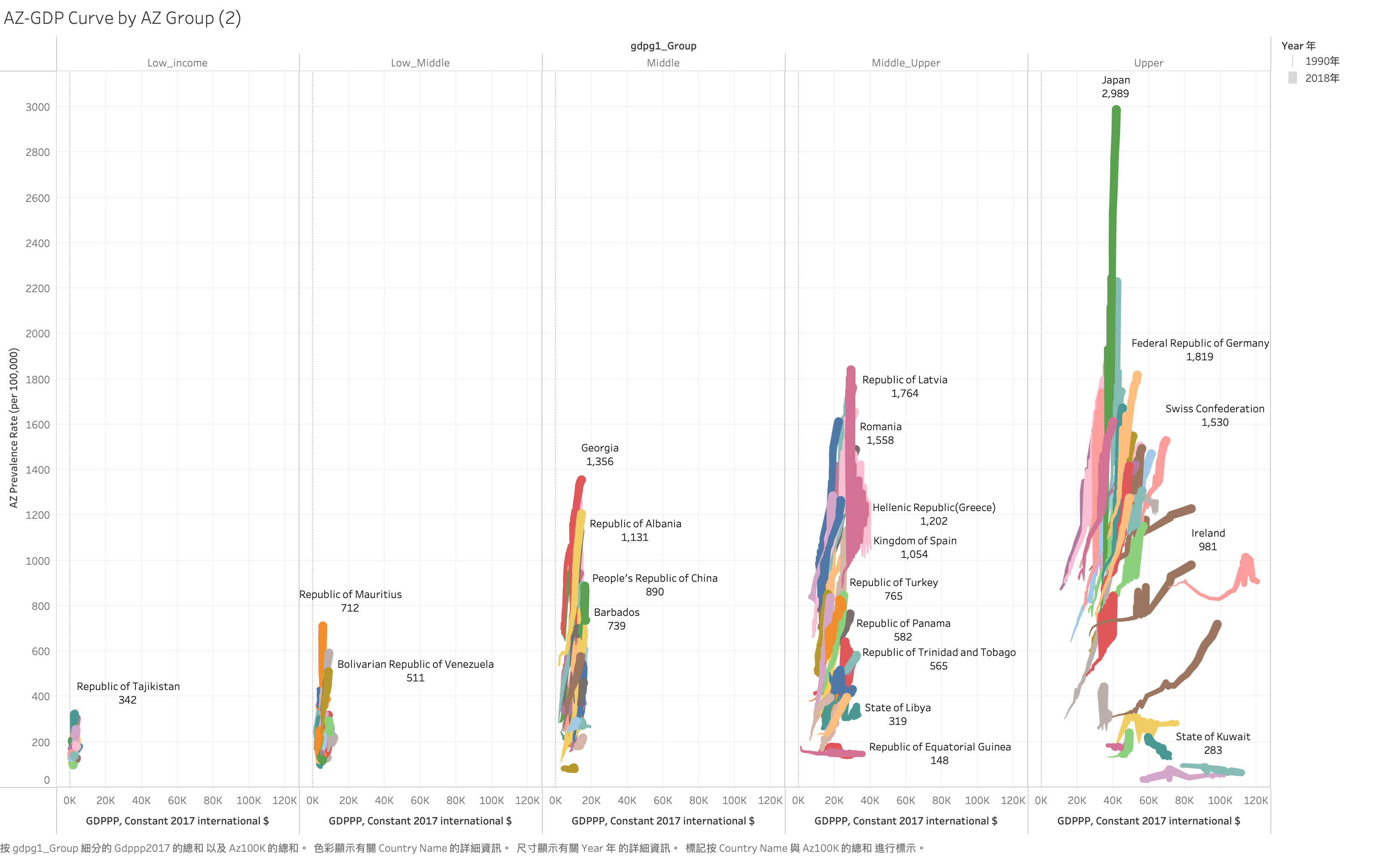
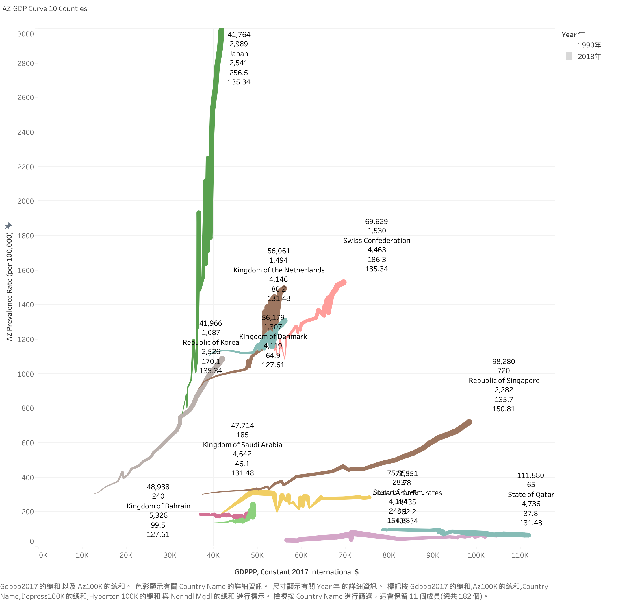
假設我們有一個數據集，包含各國的GDPPP及疾病盛行率。我們希望將這些客戶分成五個群集，步驟如下：

隨機選擇五個初始中心點。
計算每個客戶到這五個中心點的距離，將每個客戶分配給最近的中心點。
重新計算每個群集的中心點。
重複分配和更新，直到中心點不再變化。

這樣我們就可以將客戶分成五個群集，每個群集代表一組具有相似消費行為的客戶。

K-Means 是一個強大且常用的工具，但在實際應用中需要考慮其局限性和參數選擇。

實作

import numpy as np

# Import necessary libraries
from google.colab import drive
import pandas as pd
from sklearn.cluster import KMeans
from sklearn.preprocessing import StandardScaler
from sklearn.impute import SimpleImputer

# Mount Google Drive
drive.mount('/content/drive')

# Read the CSV file into a pandas DataFrame
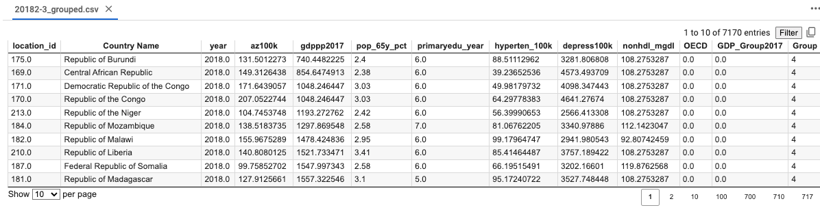
df = pd.read_csv('/content/drive/MyDrive/KMEAN/AZRV_20182_0523.csv')

# Convert the 'gdppp' column to float
df['gdppp2017'] = df['gdppp2017'].astype(float)

# Group the data by GDPPP into five groups
df['GDP_Group2017'] = pd.qcut(df['gdppp2017'], q=5, labels=False)

# Select the features
# features = ['az100k', 'pop_65y_pct', 'primaryedu_year', 'hyperten_100k','depress100K', 'nonhdl_mgdl']
features = ['az100k', 'pop_65y_pct', 'primaryedu_year', 'hyperten_100k','depress100k', 'nonhdl_mgdl']


# Only keep the GDP_Group and other features
X = df[features]

# Standardize the features
scaler = StandardScaler()
X_scaled = scaler.fit_transform(X)

# Impute missing values with the mean
imputer = SimpleImputer(strategy='mean')
X_scaled = imputer.fit_transform(X_scaled)

# Check for missing values
missing_values = np.isnan(X_scaled).sum()
print(missing_values)

# Use K-means clustering to cluster the data into five groups
kmeans = KMeans(n_clusters=5, random_state=42)
kmeans.fit(X_scaled)
labels = kmeans.labels_

# Add the cluster labels to the original data
df['Group'] = labels

# Print the summary statistics for each cluster
group_stats = df.groupby('Group')[features].describe()
print(group_stats)

# If you need to save the clustered data
df.to_csv('20182-3_grouped.csv', index=False)

Output, 分群


import numpy as np

# Import necessary libraries
from google.colab import drive
import pandas as pd
from sklearn.cluster import KMeans
from sklearn.preprocessing import StandardScaler
from sklearn.impute import SimpleImputer

# Mount Google Drive
…group_stats = df.groupby('Group')[features].describe()
print(group_stats)

# If you need to save the clustered data
df.to_csv('20182-3_grouped.csv', index=False)
Drive already mounted at /content/drive; to attempt to forcibly remount, call drive.mount("/content/drive", force_remount=True).
0
/usr/local/lib/python3.10/dist-packages/sklearn/cluster/_kmeans.py:870: FutureWarning: The default value of `n_init` will change from 10 to 'auto' in 1.4. Set the value of `n_init` explicitly to suppress the warning
  warnings.warn(
      az100k                                                                 \
       count         mean         std         min          25%          50%   
Group                                                                         
0       42.0   570.731959  279.813076   77.854194   413.589506   514.001773   
1       29.0  1357.713112  359.876139  642.569608  1229.188301  1423.406956   
2       39.0   333.656546  186.450738   87.086735   214.407278   298.565050   
3       20.0  1471.588495  504.890367  765.350228  1188.206307  1395.787605   
4       52.0   183.498420   78.811741   87.810353   135.230484   156.533061   

                                pop_65y_pct             ...  depress100k  \
               75%          max       count       mean  ...          75%   
Group                                                   ...                
0       709.346476  1316.266357        42.0   7.546905  ...  4122.836259   
1      1624.709701  1912.203997        29.0  15.430000  ...  4830.947694   
2       386.726109  1082.130196        39.0   5.138462  ...  3024.226697   
3      1661.257484  2989.455411        20.0  17.926000  ...  4384.161605   
4       197.502121   477.291516        52.0   3.234615  ...  4315.502244   

                   nonhdl_mgdl                                                 \
               max       count        mean        std         min         25%   
Group                                                                           
0      5332.211057        42.0  132.766177   8.353623  116.009281  127.610209   
1      6033.519387        29.0  135.344161   8.396135  119.876257  127.610209   
2      3749.435931        39.0  134.550935  10.503569  116.009281  127.610209   
3      5011.843218        20.0  139.984532   6.940174  127.610209  135.344161   
4      5325.835877        52.0  109.688262   7.425607   92.807425  108.275329   

                                           
              50%         75%         max  
Group                                      
0      131.477185  139.211137  158.546017  
1      131.477185  139.211137  150.812065  
2      135.344161  143.078113  162.412993  
3      143.078113  143.078113  150.812065  
4      108.275329  112.142305  131.477185  

[5 rows x 48 columns

Visualization

WDI 的 GDPPP Grouping : US$ 996, 3895,12055 , 4 Group

K-Mean clustering : GDPPP: (3513),(9,636),(16145),( 34,040 ) 5 Group