Heat MAP.MSCI 個股對 TAIEX 的 Pearson analysis.(f)0630


MSCI 個股對 TAIEX 的 Pearson analysis
import pandas as pd
import numpy as np
import matplotlib.pyplot as plt
import seaborn as sns
from scipy.stats import pearsonr
# Mount Google Drive
from google.colab import drive
drive.mount('/content/drive', force_remount=True)
# Load the data
file_path = '/content/drive/My Drive/MSCI_Taiwan_30_data.csv'
data = pd.read_csv(file_path)
# Select only numerical columns
numerical_data = data.select_dtypes(include=[np.number])
# Handle NaN and infinite values by replacing them with the mean of the column
numerical_data = numerical_data.apply(lambda x: np.where(np.isfinite(x), x, np.nan))
numerical_data = numerical_data.apply(lambda x: x.fillna(x.mean()), axis=0)
# Define the target variable
target_variable = 'Close_TAIEX'
# Extract unique stock codes and names
stock_codes = data['ST_Code'].unique()
stock_names = data[['ST_Code', 'ST_Name']].drop_duplicates().set_index('ST_Code')
# Initialize dictionaries to store the correlation results and p-values
correlation_results = {}
p_value_results = {}
# Iterate over each stock code
for stock_code in stock_codes:
# Filter the data for the specific stock
stock_data = data[data['ST_Code'] == stock_code]
numerical_stock_data = stock_data.select_dtypes(include=[np.number])
# Align the lengths of the target variable and the stock data
common_index = numerical_data.index.intersection(numerical_stock_data.index)
aligned_target = numerical_data.loc[common_index, target_variable]
aligned_stock_data = numerical_stock_data.loc[common_index]
# Handle NaN and infinite values for the aligned stock data
aligned_stock_data = aligned_stock_data.apply(lambda x: np.where(np.isfinite(x), x, np.nan))
aligned_stock_data = aligned_stock_data.apply(lambda x: x.fillna(x.mean()), axis=0)
# Calculate Pearson correlation with target variable 'Close_TAIEX'
for column in aligned_stock_data.columns:
if column != target_variable:
correlation, p_value = pearsonr(aligned_target, aligned_stock_data[column])
correlation_results[(stock_names.loc[stock_code, 'ST_Name'], column)] = correlation
p_value_results[(stock_names.loc[stock_code, 'ST_Name'], column)] = p_value
# Convert results to DataFrame for better visualization
correlation_df = pd.DataFrame.from_dict(correlation_results, orient='index', columns=['Pearson Correlation']).reset_index()
correlation_df[['Stock Name', 'Variable']] = pd.DataFrame(correlation_df['index'].tolist(), index=correlation_df.index)
correlation_df = correlation_df.drop(columns=['index'])
p_value_df = pd.DataFrame.from_dict(p_value_results, orient='index', columns=['P-Value']).reset_index()
p_value_df[['Stock Name', 'Variable']] = pd.DataFrame(p_value_df['index'].tolist(), index=p_value_df.index)
p_value_df = p_value_df.drop(columns=['index'])
# Merge correlation and p-value DataFrames
merged_df = pd.merge(correlation_df, p_value_df, on=['Stock Name', 'Variable'])
# Filter for significant correlations (P < 0.05)
significant_df = merged_df[merged_df['P-Value'] < 0.05]
# Pivot the DataFrame for all correlations
correlation_pivot = correlation_df.pivot_table(index='Variable', columns='Stock Name', values='Pearson Correlation')
# Pivot the DataFrame for significant correlations
significant_pivot = significant_df.pivot_table(index='Variable', columns='Stock Name', values='Pearson Correlation')
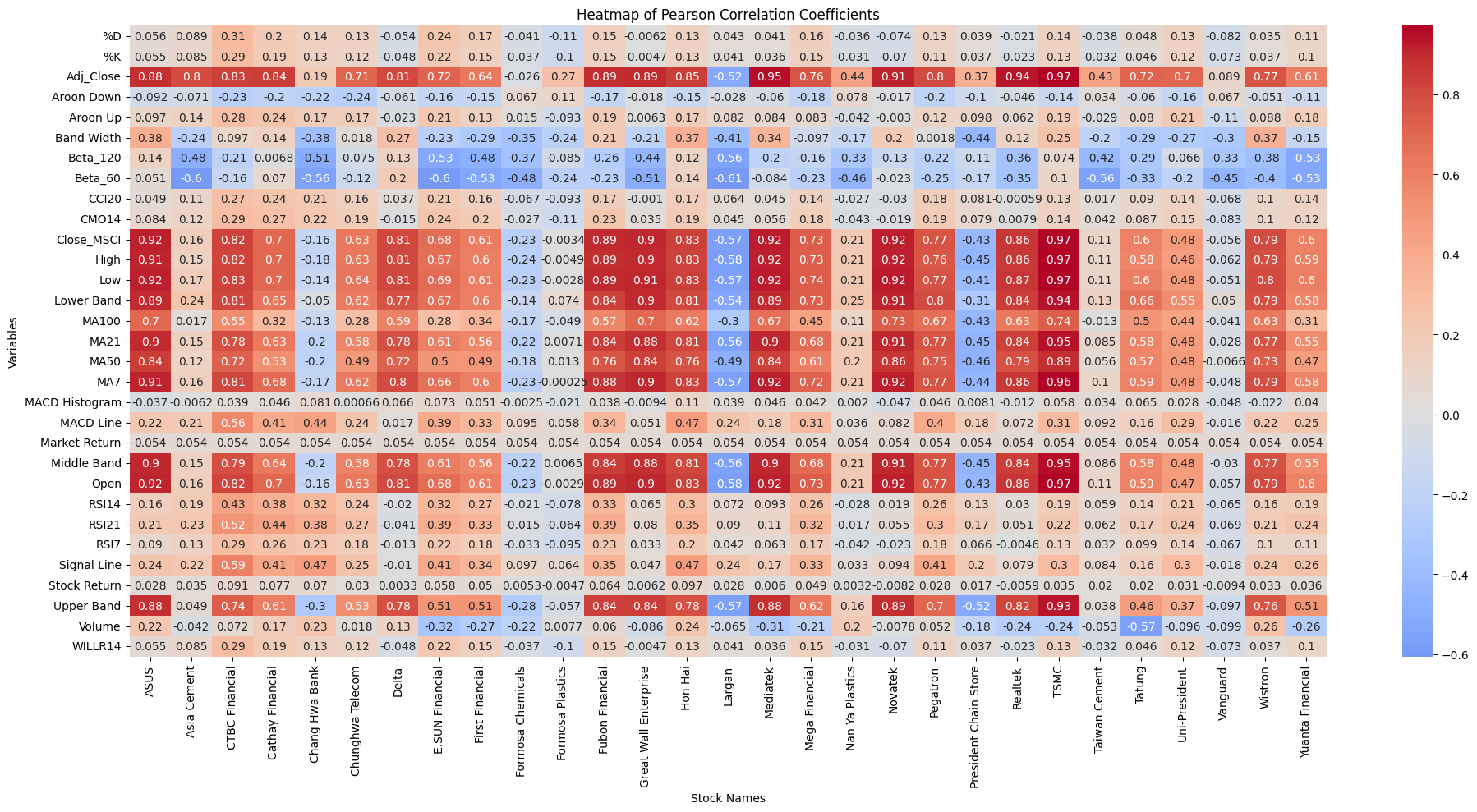
# Plot heatmap for all correlations
plt.figure(figsize=(20, 10))
sns.heatmap(correlation_pivot, annot=True, cmap='coolwarm', center=0)
plt.title('Heatmap of Pearson Correlation Coefficients')
plt.xlabel('Stock Names')
plt.ylabel('Variables')
plt.xticks(rotation=90)
plt.yticks(rotation=0)
plt.tight_layout()
plt.show()
# Plot heatmap for significant correlations (P < 0.05)
plt.figure(figsize=(20, 10))
sns.heatmap(significant_pivot, annot=True, cmap='coolwarm', center=0)
plt.title('Heatmap of Significant Pearson Correlation Coefficients (P < 0.05)')
plt.xlabel('Stock Names')
plt.ylabel('Variables')
plt.xticks(rotation=90)
plt.yticks(rotation=0)
plt.tight_layout()
plt.show()
import pandas as pd import yfinance as yf import ta from datetime import datetime
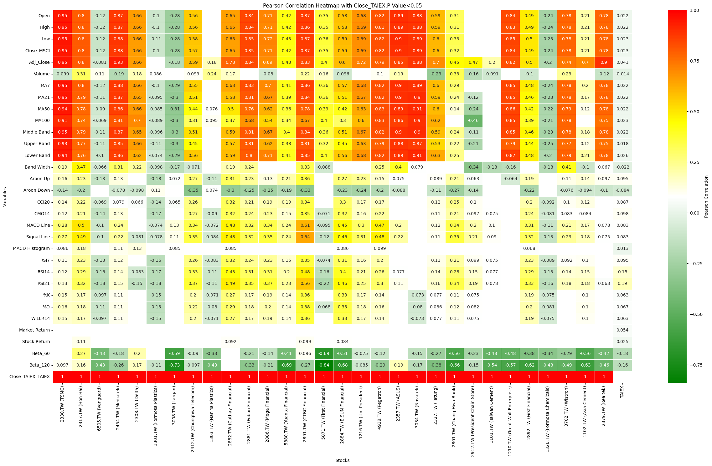
Heat Map, Pearson's analysis, P<0.05,Code
import pandas as pd
import numpy as np
import seaborn as sns
import matplotlib.pyplot as plt
from scipy.stats import pearsonr
from matplotlib.colors import LinearSegmentedColormap

# Mount Google Drive
from google.colab import drive
drive.mount('/content/drive', force_remount=True)

# Load the data
file_path = '/content/drive/My Drive/MSCI_Taiwan_30_data.csv'
data = pd.read_csv(file_path)

# Convert 'Date' column to datetime
data['Date'] = pd.to_datetime(data['Date'], format='%Y/%m/%d')

# Define the target variable
target_variable = 'Close_TAIEX'

# Calculate Pearson correlation and p-values
def calculate_pearson_correlation(data, target_variable):
    correlation_results = {}
    numerical_columns = data.select_dtypes(include=[np.number]).columns

    for column in numerical_columns:
        if column != target_variable:
            cleaned_data = data[[target_variable, column]].dropna()
            if cleaned_data.shape[0] > 0:
                correlation, p_value = pearsonr(cleaned_data[target_variable], cleaned_data[column])
                if p_value <= 0.05:
                    correlation_results[column] = correlation
                else:
                    correlation_results[column] = np.nan
            else:
                correlation_results[column] = np.nan

    return correlation_results

# Initialize an empty DataFrame to store correlation results
correlation_df = pd.DataFrame()

# Iterate over each unique stock code
for stock_code in data['ST_Code'].unique():
    stock_data = data[data['ST_Code'] == stock_code].copy()
    taiex_data = data[['Date', target_variable]].drop_duplicates().copy()

    # Align indices by merging on 'Date'
    aligned_data = pd.merge(stock_data, taiex_data, on='Date', suffixes=('', '_TAIEX'))
    if aligned_data.shape[0] == 0:
        print(f"No overlapping dates found for {stock_code} and {target_variable}.")
        continue

    # Handle NaN and infinite values by replacing them with the mean of the column
    aligned_data = aligned_data.replace([np.inf, -np.inf], np.nan)
    aligned_data = aligned_data.dropna()

    # Calculate Pearson correlation for the aligned data
    correlation_results = calculate_pearson_correlation(aligned_data, target_variable)
    stock_name = aligned_data['ST_Name'].iloc[0]
    correlation_df[f'{stock_code} ({stock_name})'] = pd.Series(correlation_results)

# Add TAIEX to the correlation DataFrame
taiex_correlation = calculate_pearson_correlation(data, target_variable)
correlation_df['TAIEX'] = pd.Series(taiex_correlation)

# Custom colormap
cmap = LinearSegmentedColormap.from_list(
    'custom_cmap',
    [(0, 'green'), (0.5, 'white'), (0.7, 'yellow'), (1, 'red')]
)

# Plot heatmap with swapped axes
plt.figure(figsize=(25, 15))
sns.heatmap(correlation_df, annot=True, cmap=cmap, linewidths=0.5, linecolor='white', cbar_kws={'label': 'Pearson Correlation'})
plt.title('Pearson Correlation Heatmap with Close_TAIEX')
plt.ylabel('Variables')
plt.xlabel('Stocks')
plt.xticks(rotation=90)
plt.yticks(rotation=0)
plt.tight_layout()
plt.savefig('/content/drive/My Drive/pearson_correlation_heatmap_swapped_axes.png')
plt.show()
import pandas as pd import yfinance as yf import ta from datetime import datetime