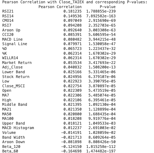
MSCI.TW30.Pearson correlation coefficient,Draft,發散的亂算

import pandas as pd
import numpy as np
import matplotlib.pyplot as plt
import seaborn as sns
from scipy.stats import pearsonr
# Mount Google Drive
from google.colab import drive
drive.mount('/content/drive', force_remount=True)
# Load the data
file_path = '/content/drive/My Drive/MSCI_Taiwan_30_data.csv'
data = pd.read_csv(file_path)
# Select only numerical columns
numerical_data = data.select_dtypes(include=[np.number])
# Handle NaN and infinite values by replacing them with the mean of the column
numerical_data = numerical_data.apply(lambda x: np.where(np.isfinite(x), x, np.nan))
numerical_data = numerical_data.apply(lambda x: x.fillna(x.mean()), axis=0)
# Calculate Pearson correlation with target variable 'Close_TAIEX'
target_variable = 'Close_TAIEX'
correlation_results = {}
for column in numerical_data.columns:
if column != target_variable:
correlation, p_value = pearsonr(numerical_data[target_variable], numerical_data[column])
correlation_results[column] = {'Pearson Correlation': correlation, 'P-value': p_value}
# Convert results to DataFrame for better visualization
correlation_df = pd.DataFrame.from_dict(correlation_results, orient='index')
correlation_df = correlation_df.sort_values(by='Pearson Correlation', ascending=False)
print("Pearson Correlation with Close_TAIEX and corresponding P-values:")
print(correlation_df)
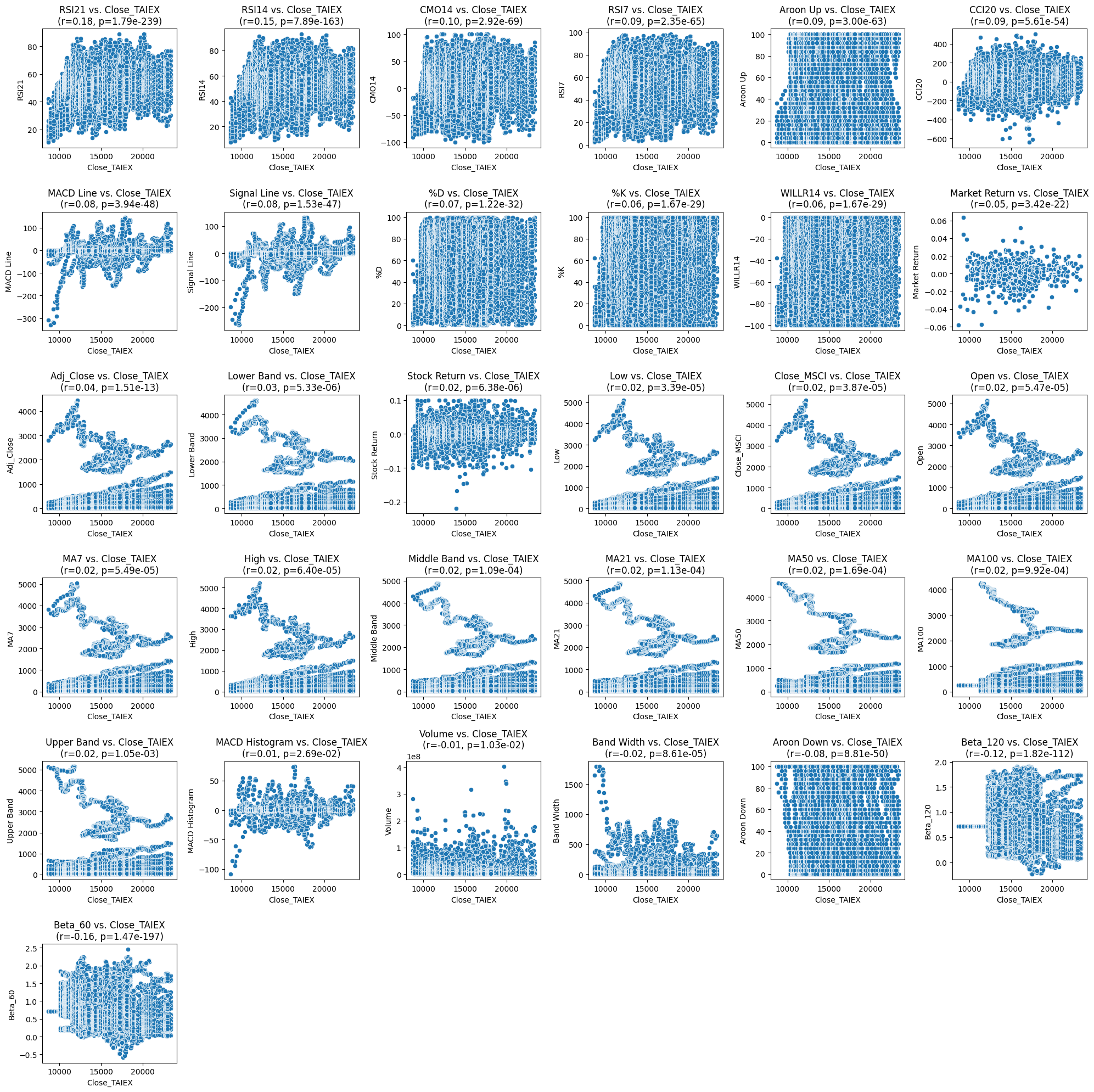
# Plot scatter plots for each explanatory variable vs. Close_TAIEX
plt.figure(figsize=(20, 20))
for i, column in enumerate(correlation_df.index):
plt.subplot(6, 6, i + 1) # Adjust the number of rows and columns based on the number of variables
sns.scatterplot(x=numerical_data[target_variable], y=numerical_data[column])
plt.title(f'{column} vs. {target_variable}\n(r={correlation_df.loc[column, "Pearson Correlation"]:.2f}, p={correlation_df.loc[column, "P-value"]:.2e})')
plt.xlabel(target_variable)
plt.ylabel(column)
plt.tight_layout()
plt.show()
import pandas as pd import yfinance as yf import ta from datetime import datetime
# Import necessary libraries
import pandas as pd
import numpy as np
import matplotlib.pyplot as plt
import seaborn as sns

# Mount Google Drive
from google.colab import drive
drive.mount('/content/drive')

# Load the data
file_path = '/content/drive/My Drive/MSCI_Taiwan_30_data.csv'
data = pd.read_csv(file_path)

# Descriptive statistics
desc_stats = data.describe()
print("Descriptive Statistics:")
print(desc_stats)

# Box plot to visualize distribution and check for outliers
plt.figure(figsize=(16, 10))
sns.boxplot(data=data.select_dtypes(include=[np.number]))  # Only plot numerical columns
plt.xticks(rotation=90)
plt.title('Box Plot of Features')
plt.show()

# Pearson correlation coefficient
numerical_data = data.select_dtypes(include=[np.number])  # Select only numerical columns
correlation_matrix = numerical_data.corr(method='pearson')

# Heatmap to visualize correlation between variables
plt.figure(figsize=(16, 10))
sns.heatmap(correlation_matrix, annot=True, fmt='.2f', cmap='coolwarm')
plt.title('Heatmap of Pearson Correlation Coefficients')
plt.show()
import pandas as pd import yfinance as yf import ta from datetime import datetime
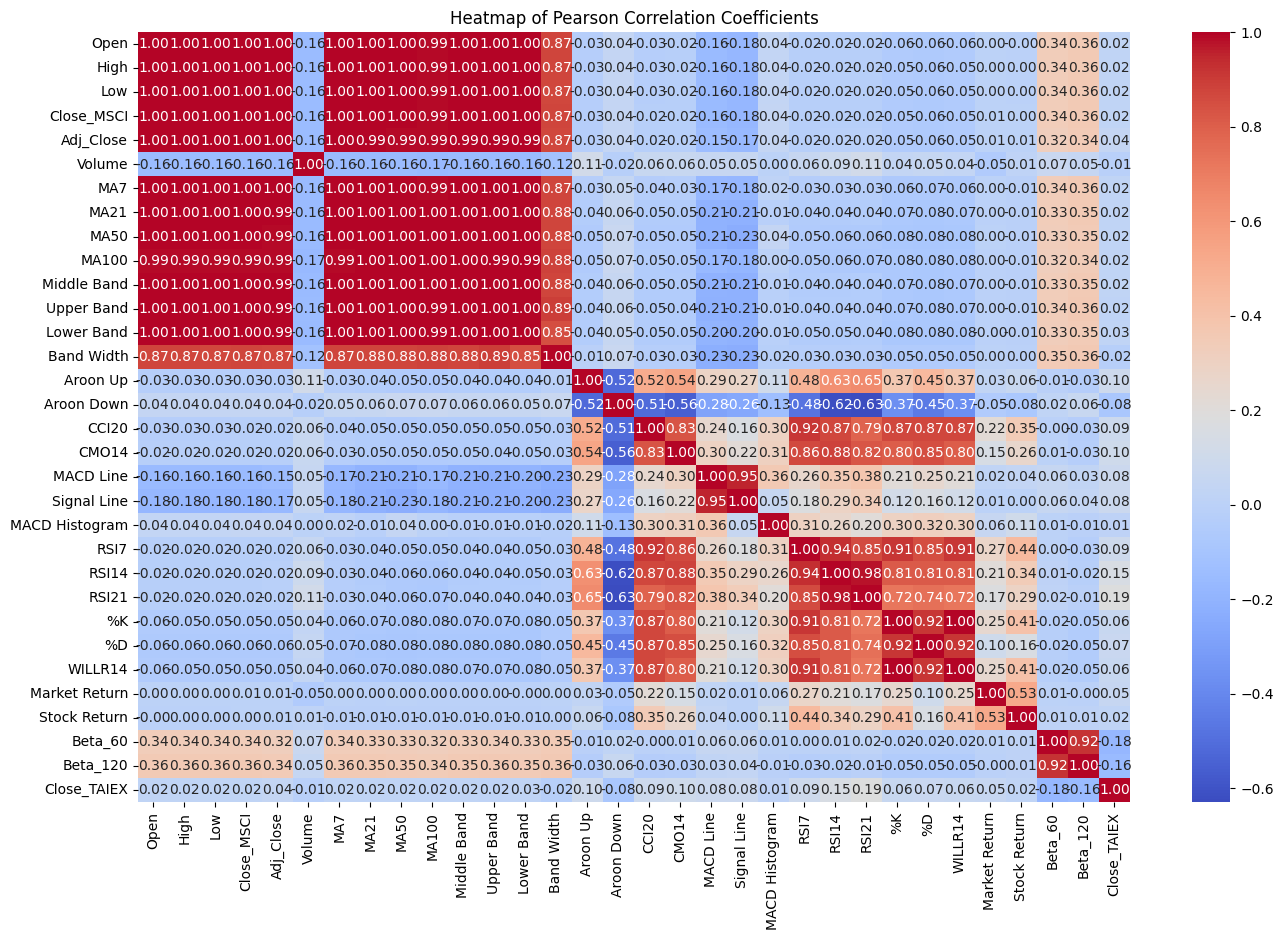
主要觀察點
- 高度正相關:
Open、High、Low、Close_MSCI、Adj_Close這些價格相關變量之間幾乎具有完全的正相關(相關係數接近1)。- 移動平均線(MA7、MA21、MA50、MA100)之間也有很高的正相關。
- 強烈相關的技術指標:
RSI14和RSI21之間有很高的正相關(0.94),表明這兩個指標在不同時間窗口下的計算結果非常相似。MACD Line和Signal Line之間的相關性也很高(0.85),這與這些指標的計算方式有關。
- 負相關:
- 一些技術指標之間存在負相關。例如,
Aroon Up和Aroon Down之間的相關性為 -0.63,這是符合邏輯的,因為這兩個指標代表了相反的市場趨勢。 Close_TAIEX和Beta_60之間有弱負相關(-0.16),這表明當Beta_60增加時,Close_TAIEX可能會減少,但這種影響較弱。
- 一些技術指標之間存在負相關。例如,