Mounted at /content/drive
Overall Pearson Correlation with Close_TAIEX:
Pearson Correlation P-value
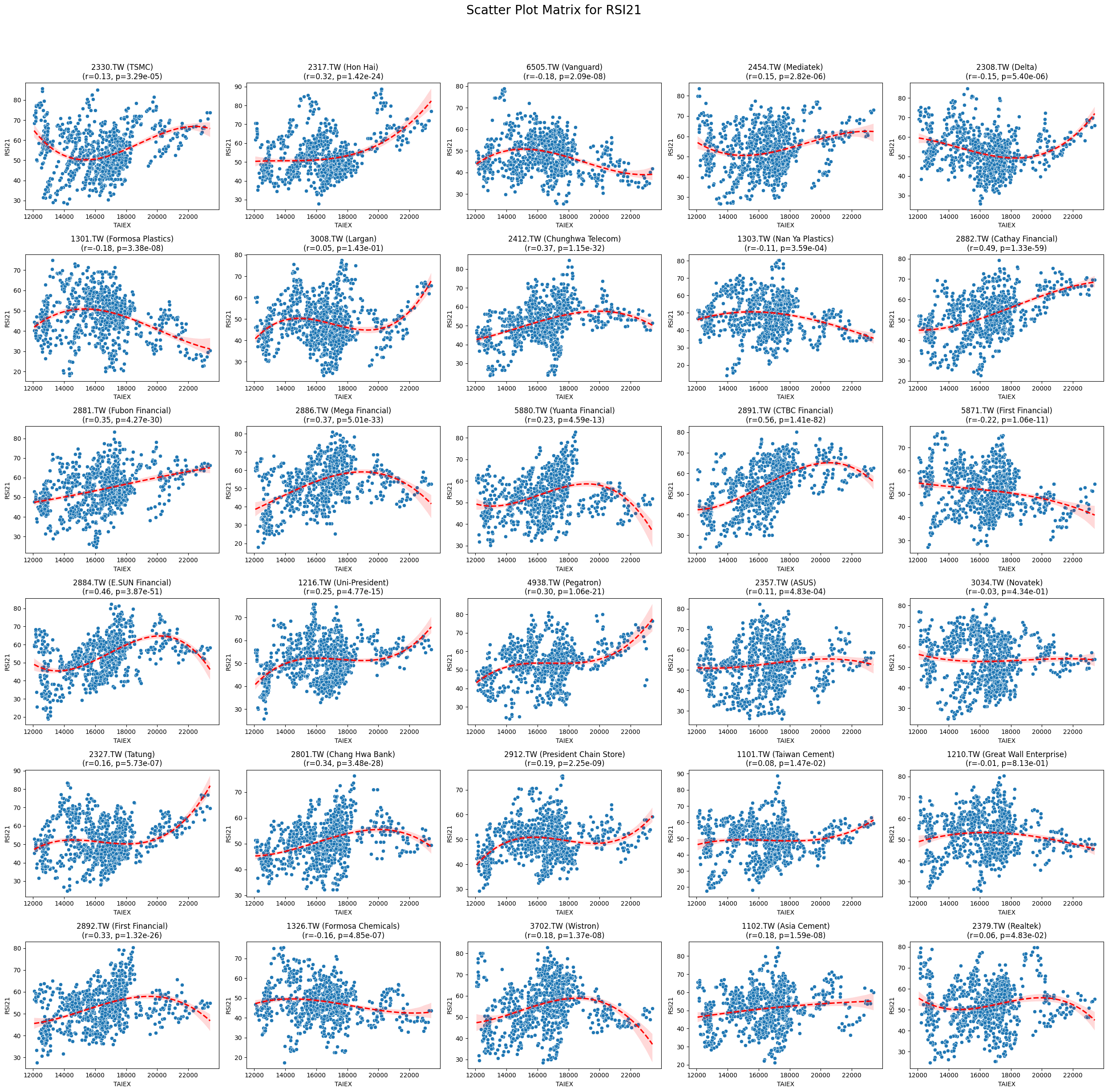
RSI21 0.185104 2.388407e-245
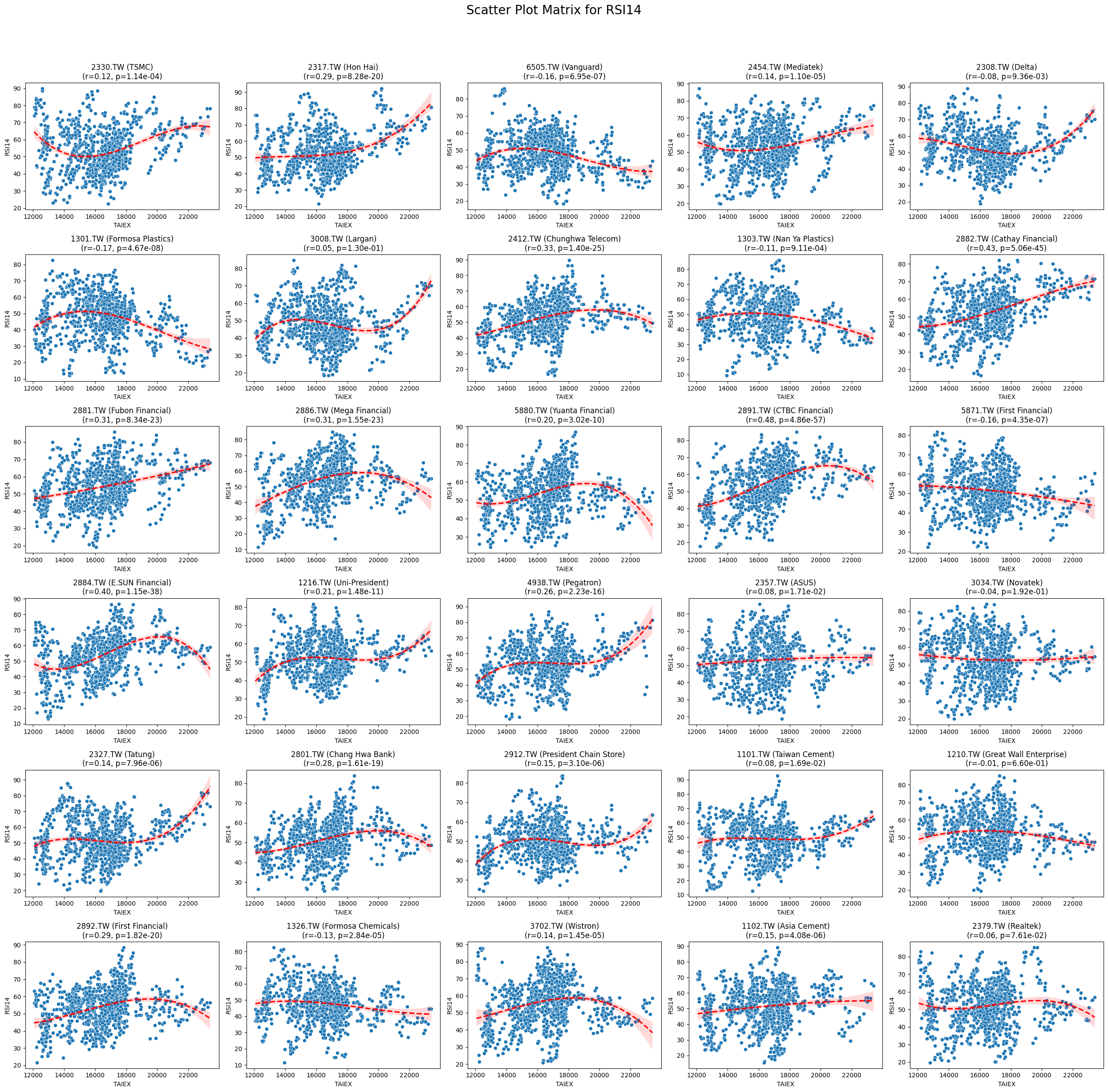
RSI14 0.151384 6.581929e-165
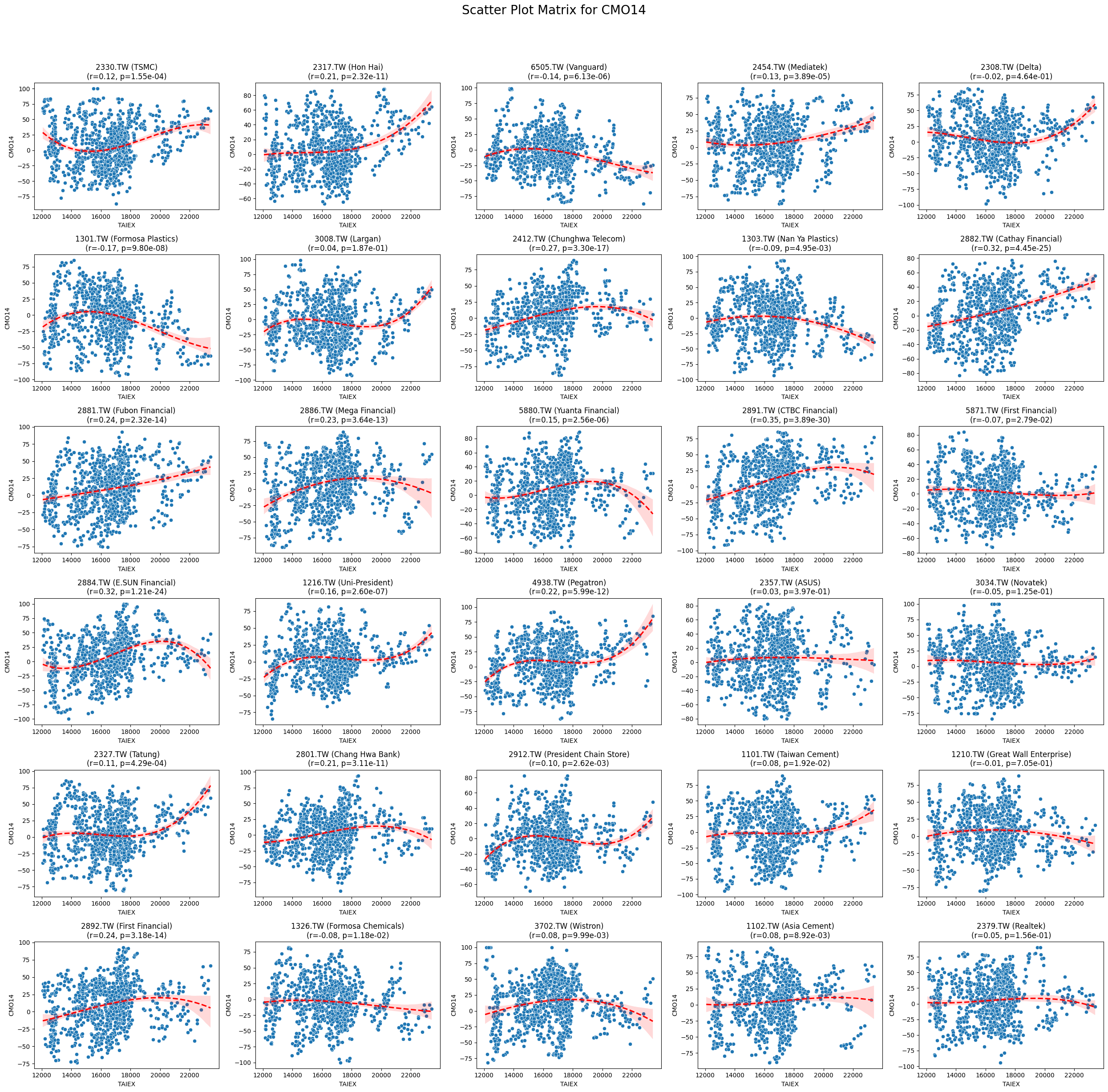
CMO14 0.098249 4.022700e-70
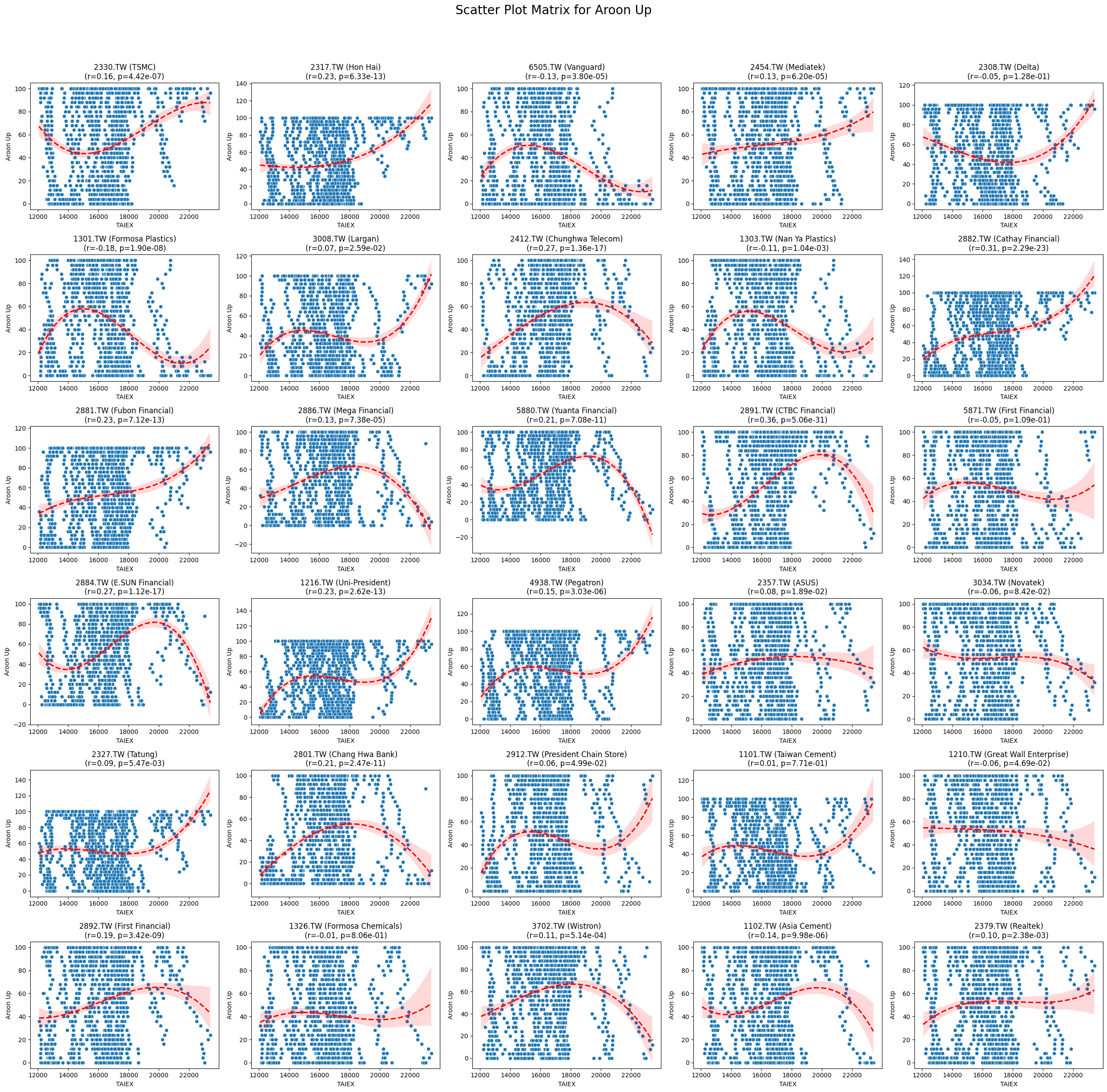
Aroon Up 0.095180 3.432801e-65
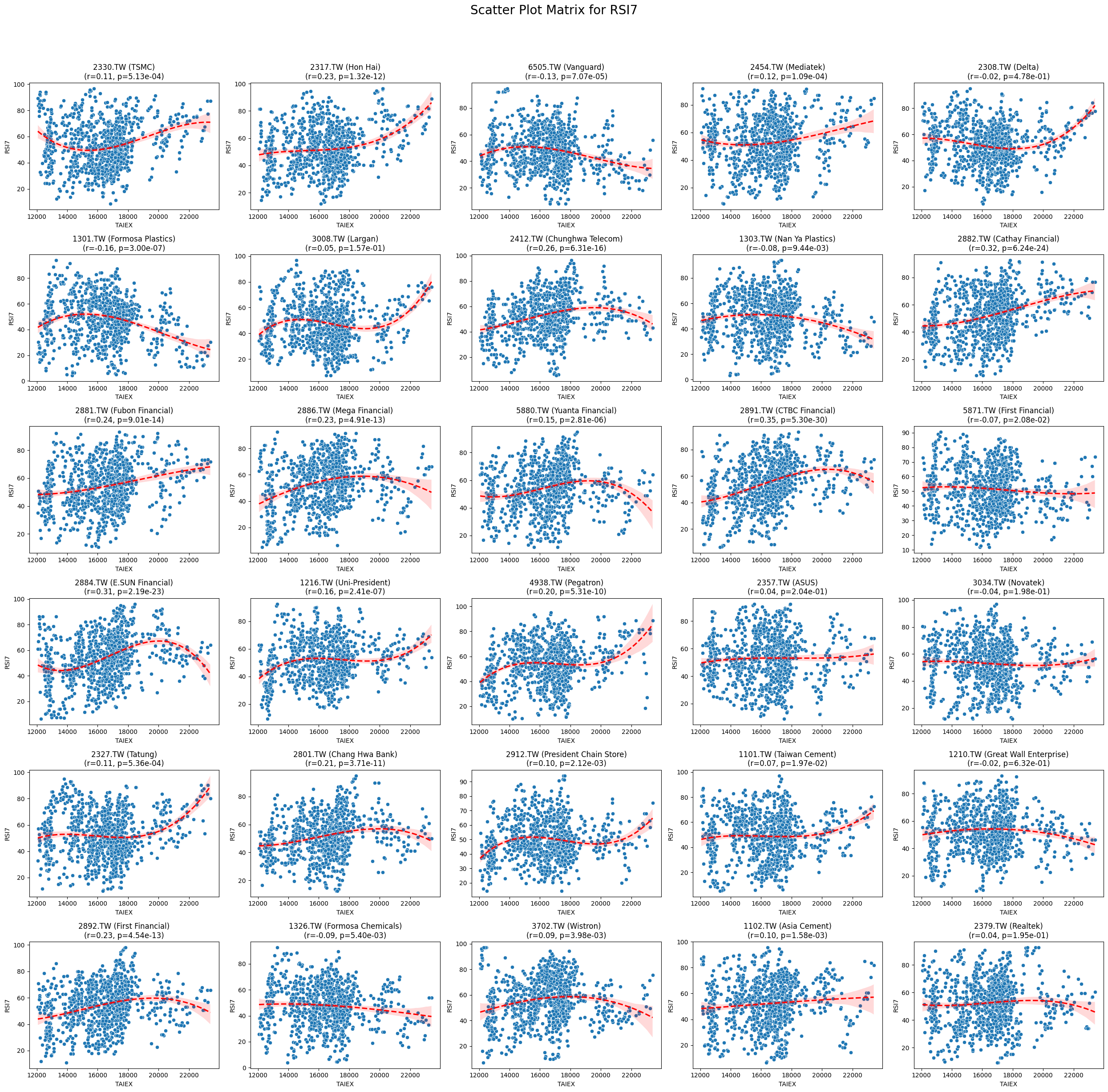
RSI7 0.094756 9.565736e-66
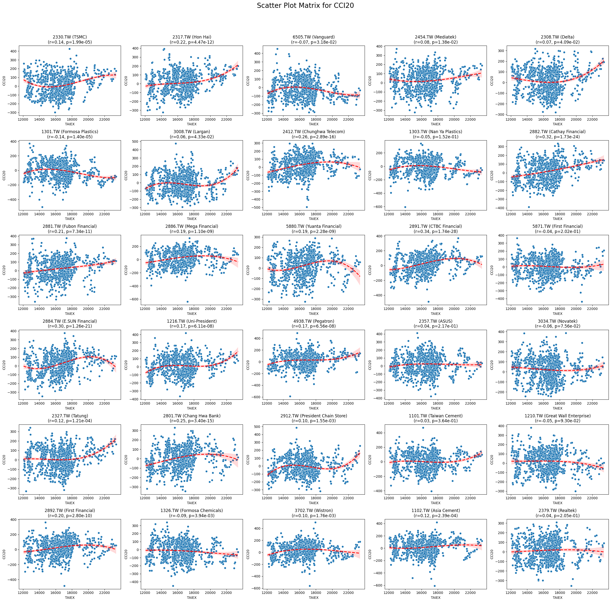
CCI20 0.087107 3.717489e-55
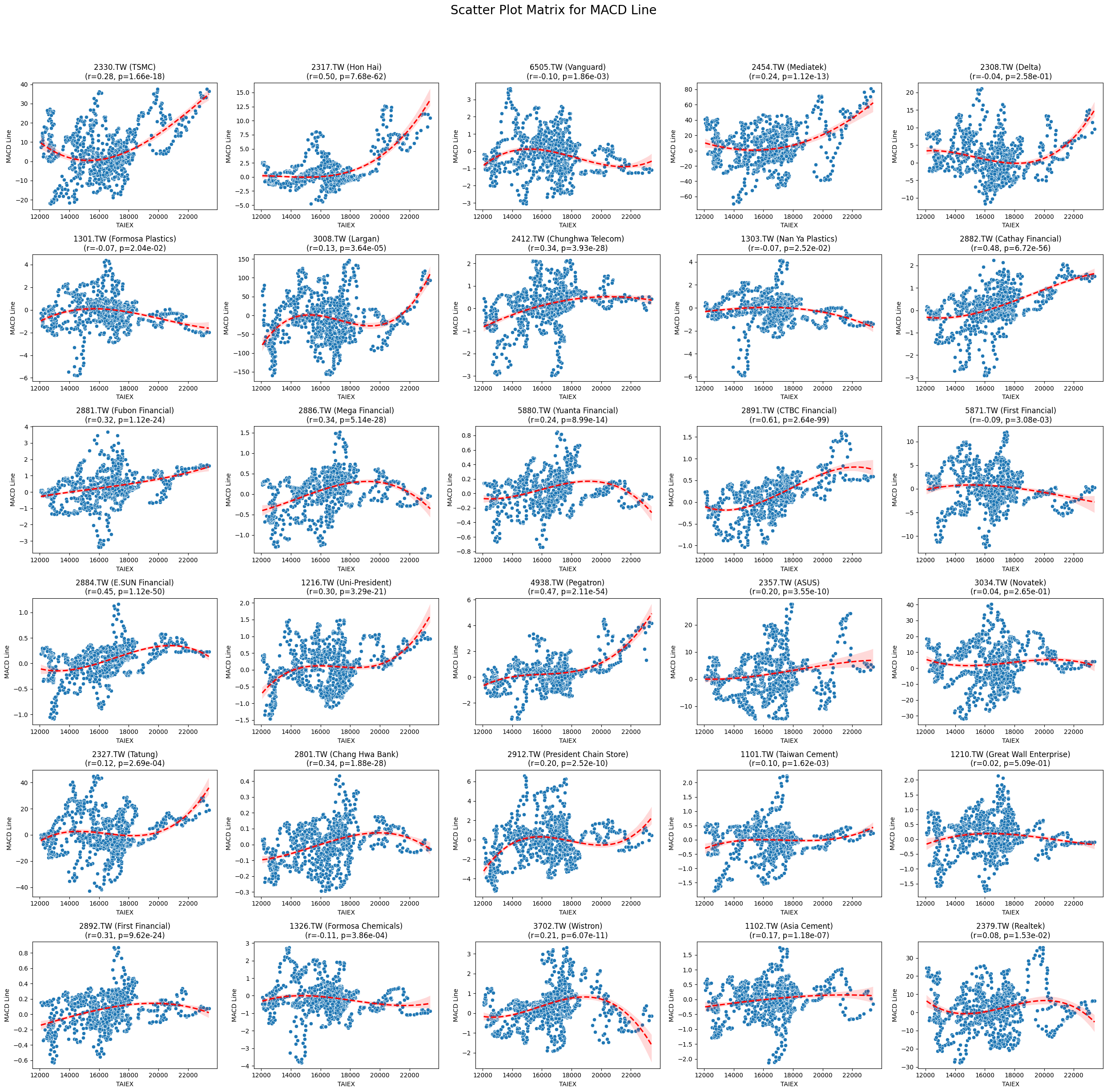
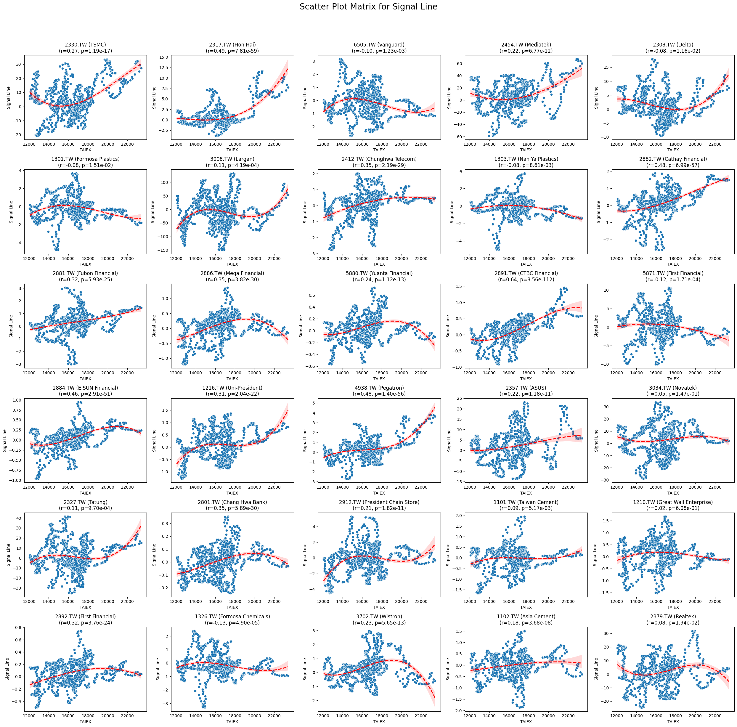
Signal Line 0.083004 1.343307e-49
MACD Line 0.082689 1.358365e-49
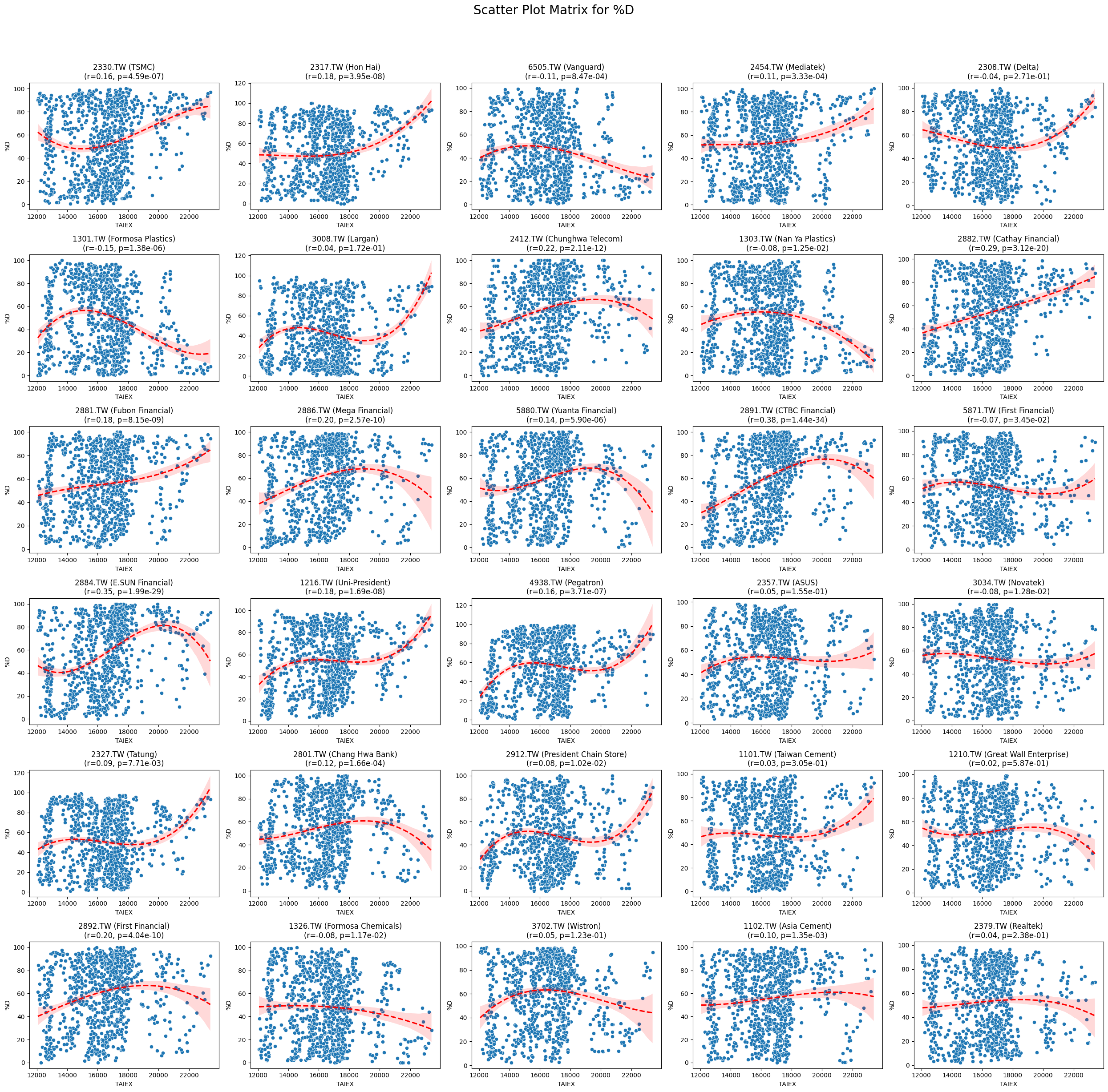
%D 0.066708 3.890501e-33
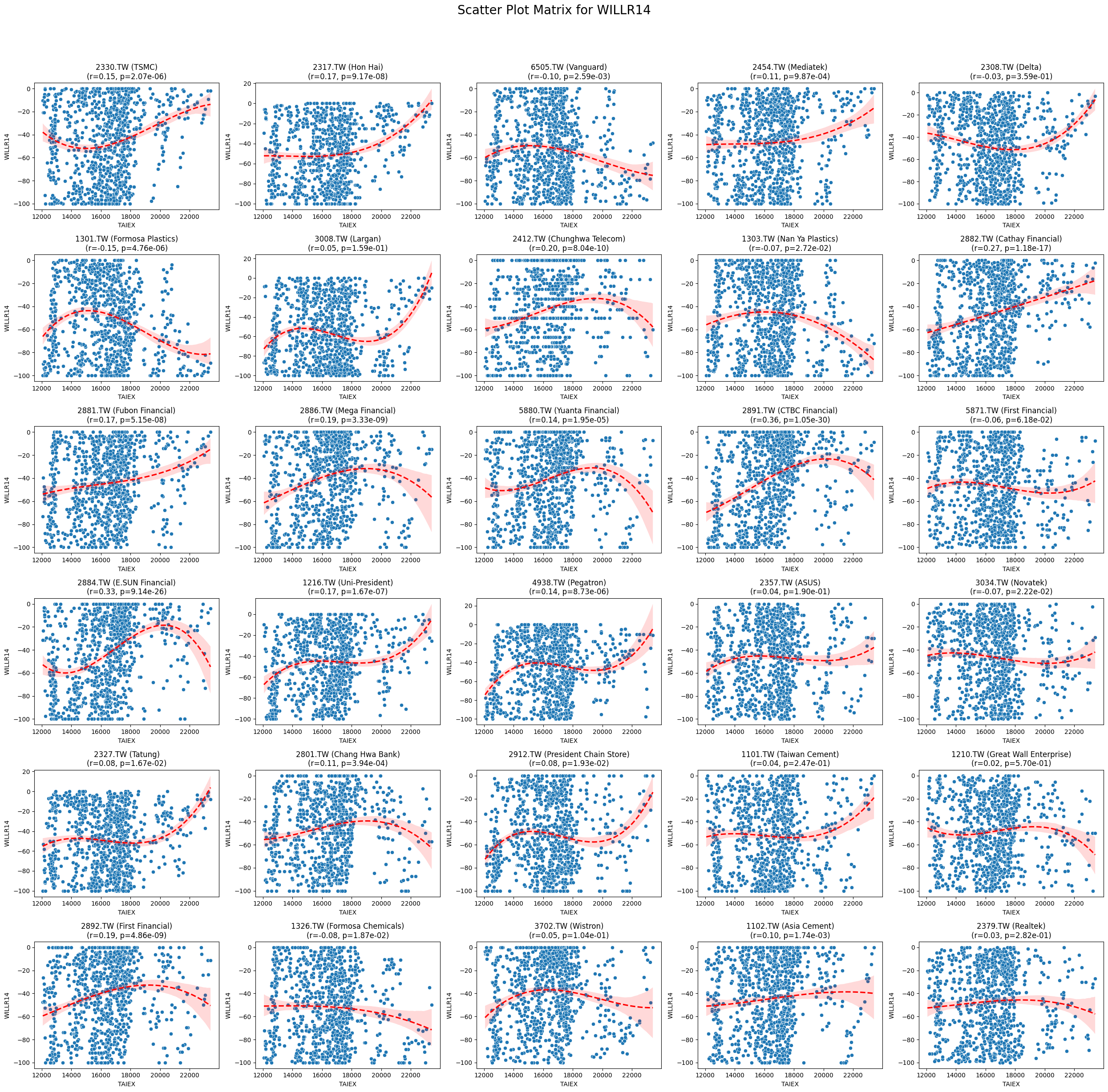
WILLR14 0.063084 7.404786e-30
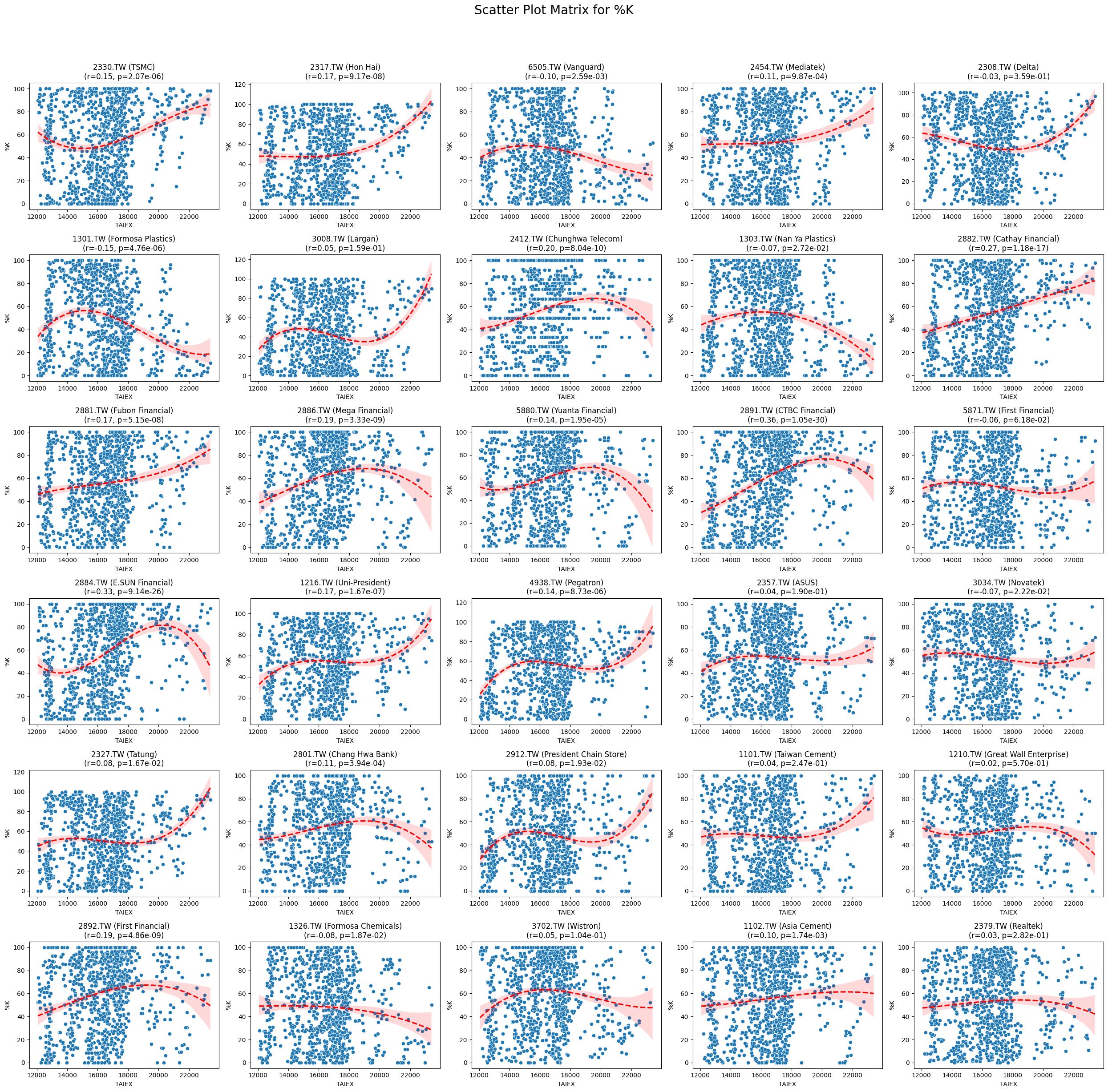
%K 0.063084 7.404786e-30
Market Return 0.053582 3.279364e-22
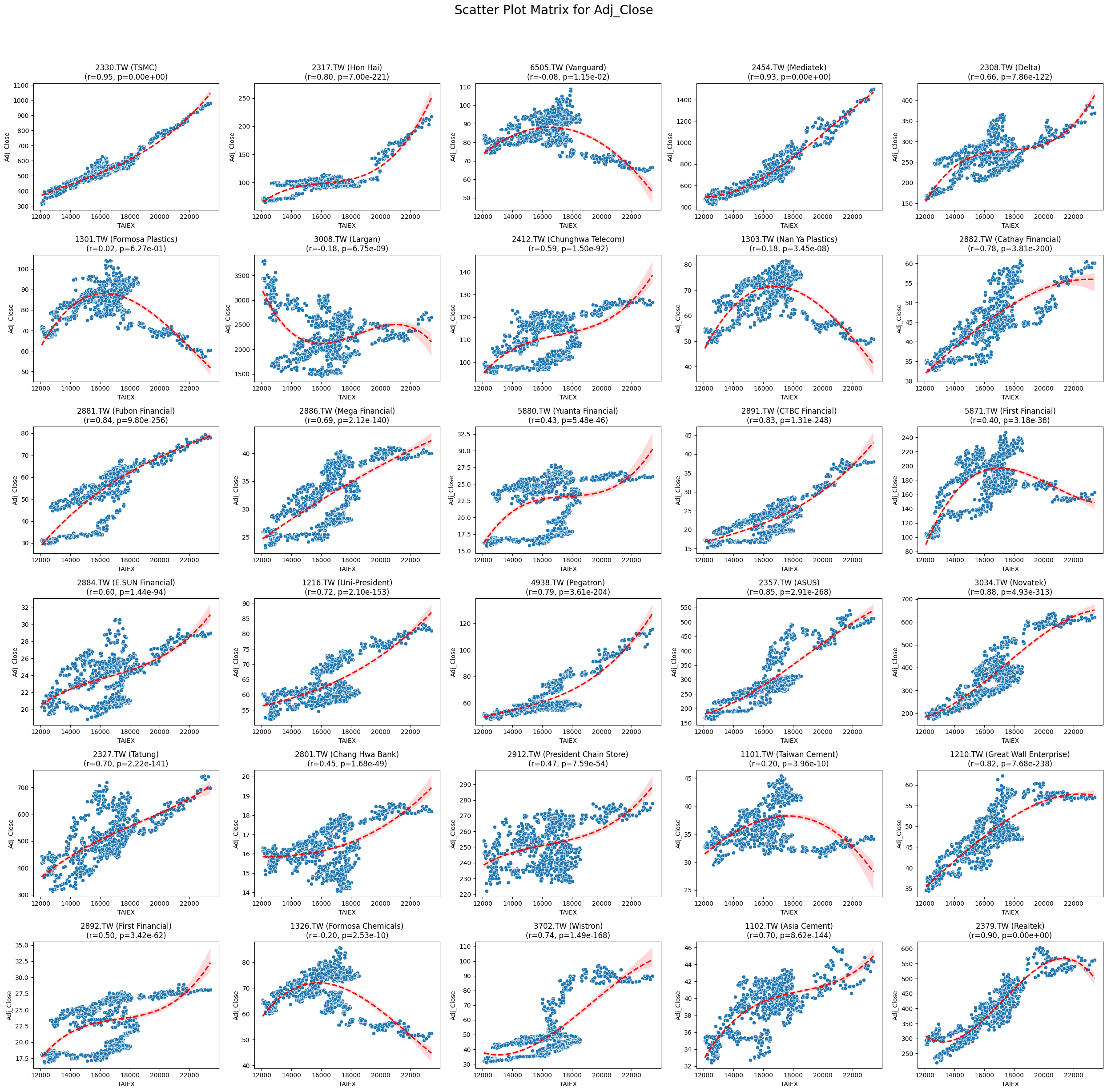
Adj_Close 0.040832 1.508200e-13
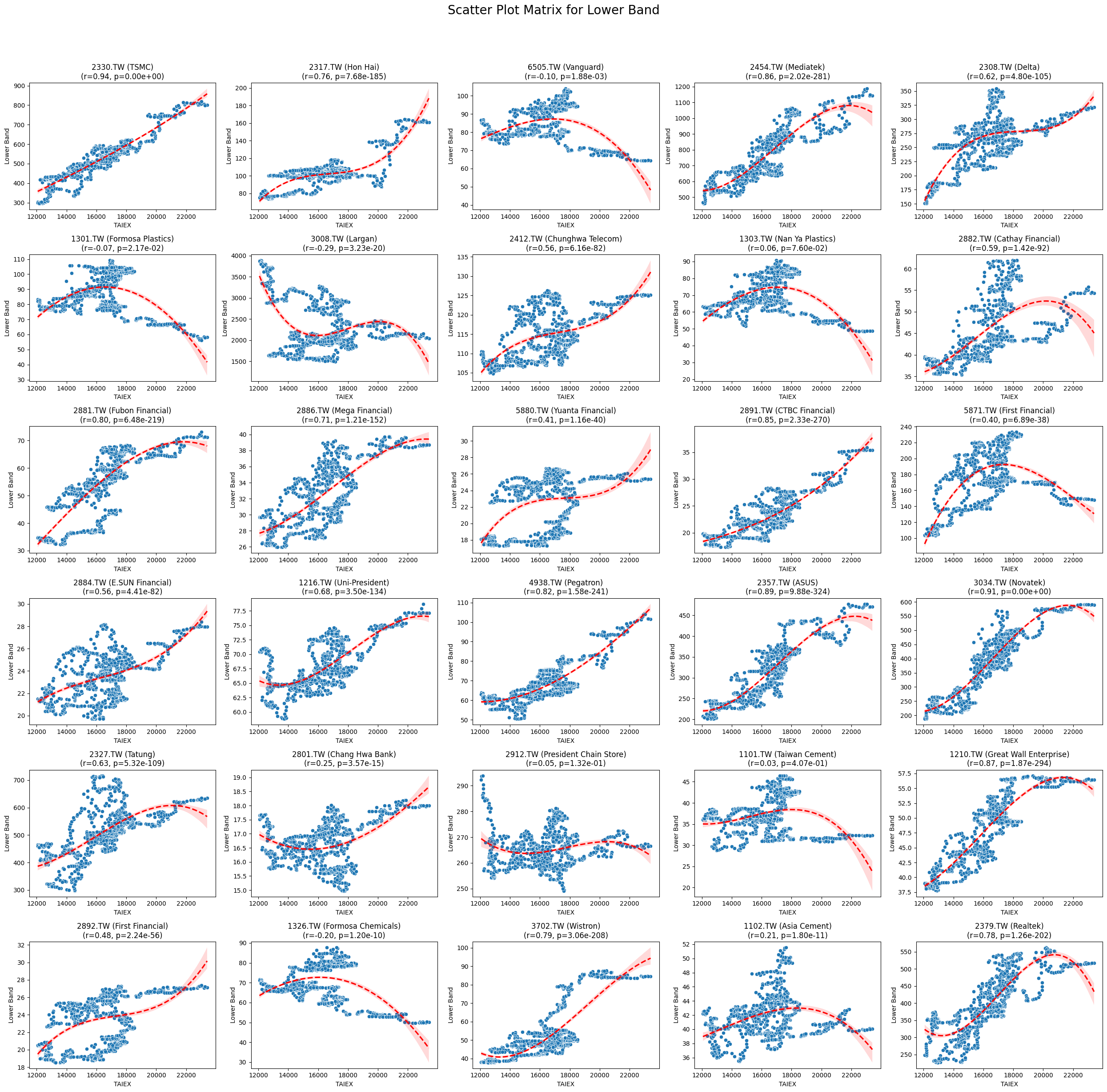
Lower Band 0.025671 4.182478e-06
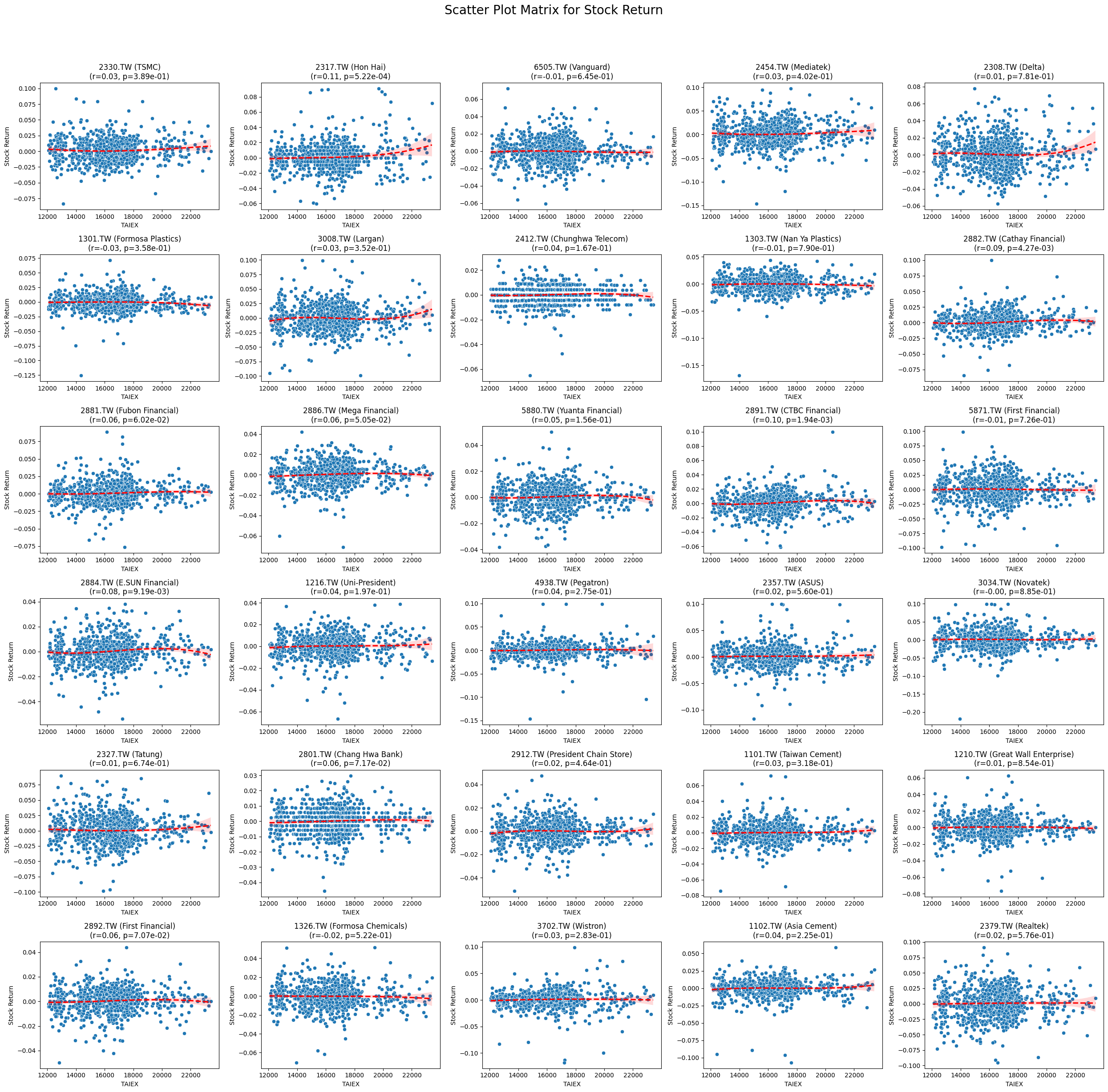
Stock Return 0.024979 6.320338e-06
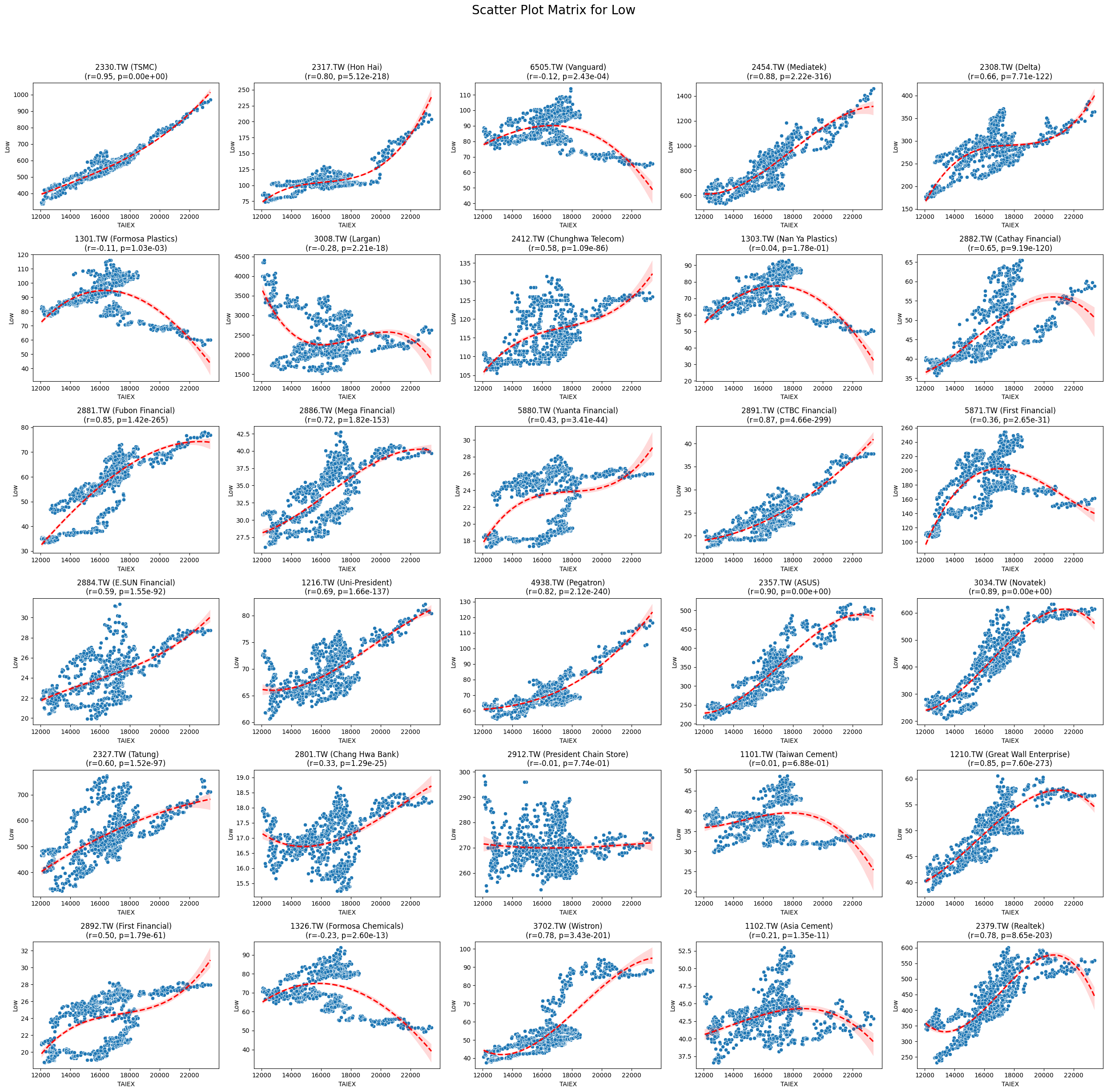
Low 0.022923 3.390795e-05
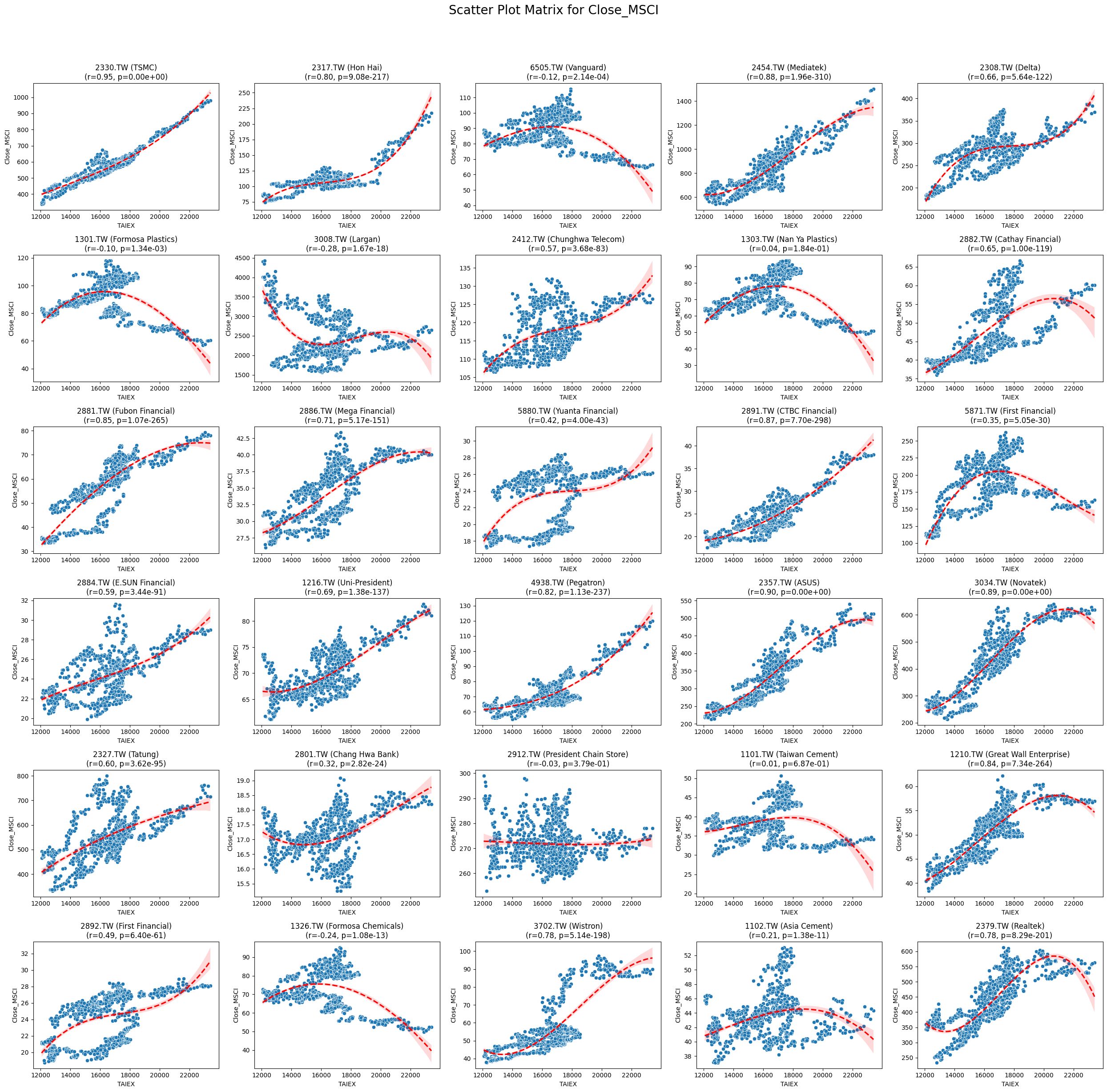
Close_MSCI 0.022754 3.870897e-05
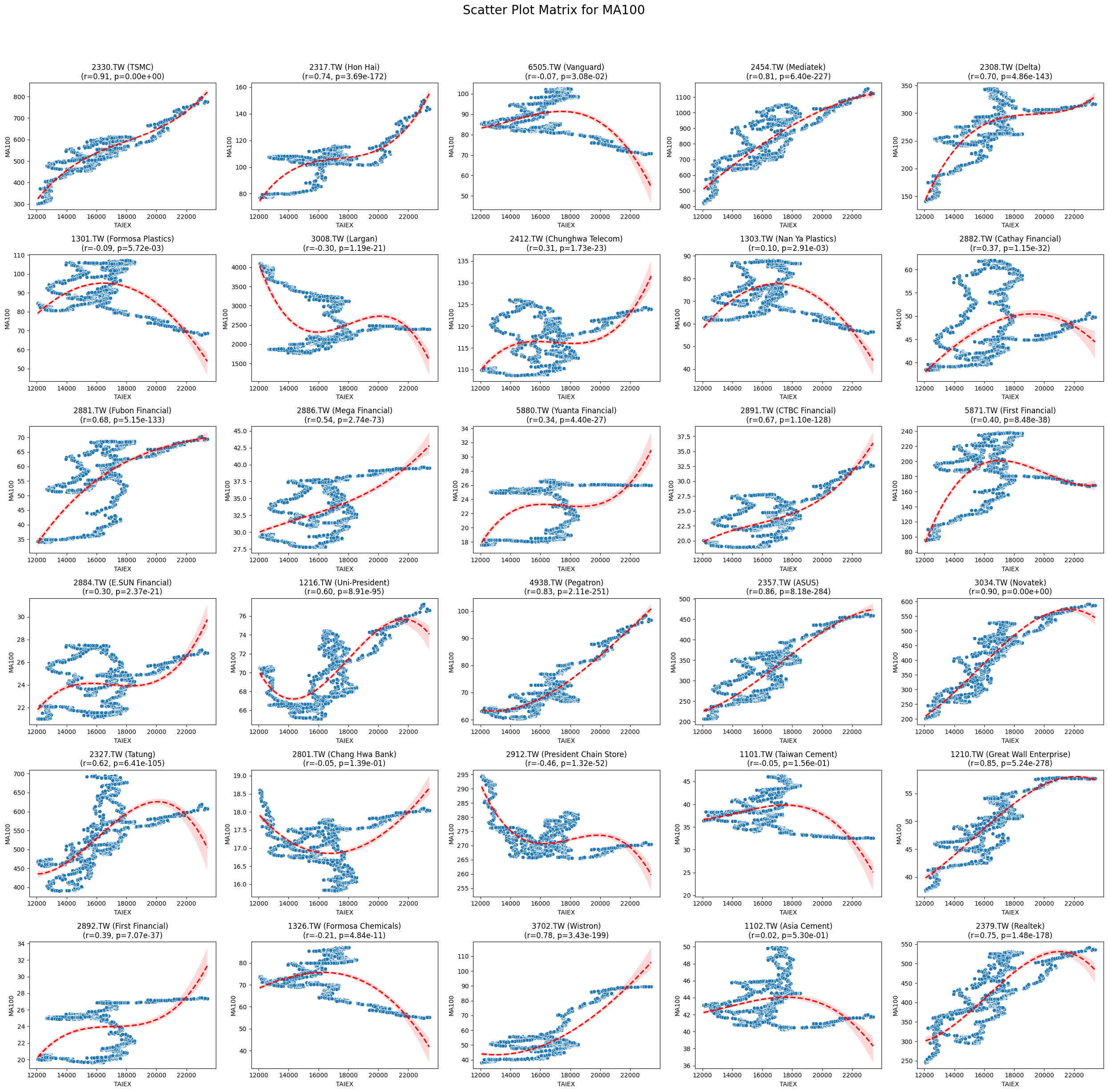
MA100 0.022563 9.995018e-05
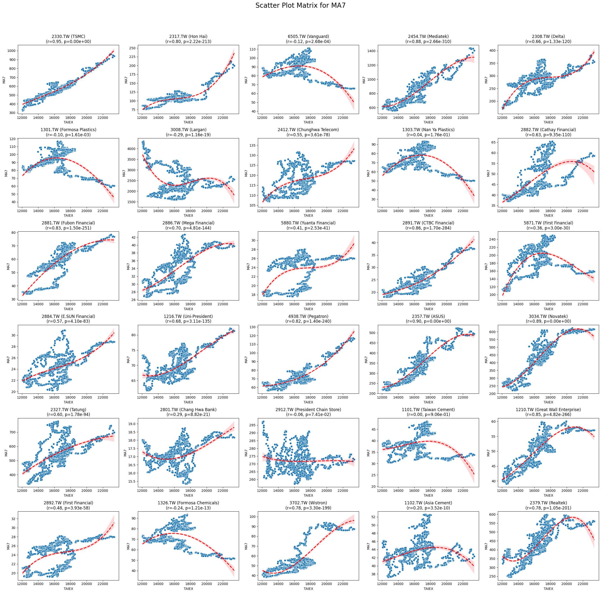
MA7 0.022436 5.204963e-05
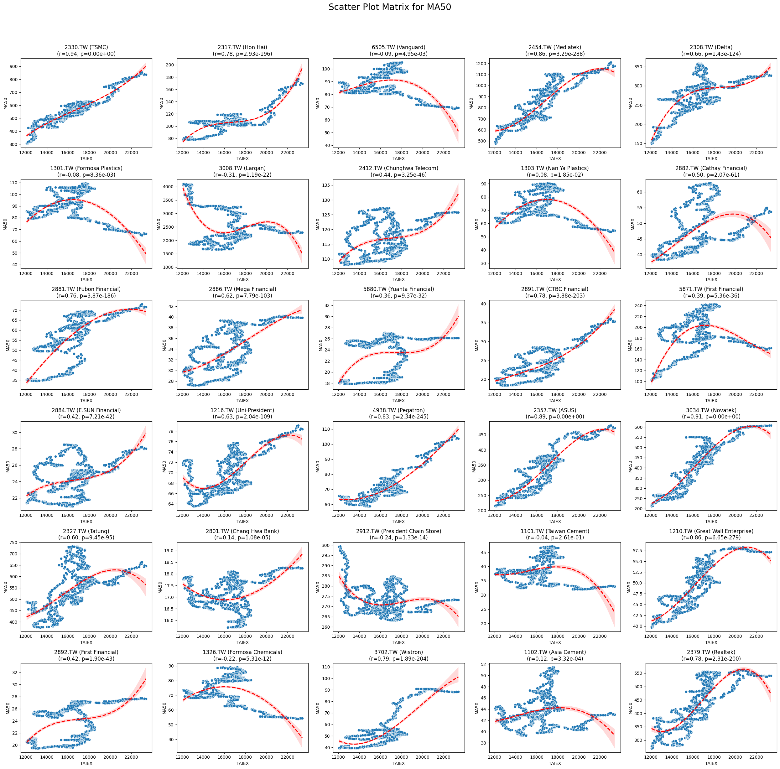
MA50 0.022385 7.611907e-05
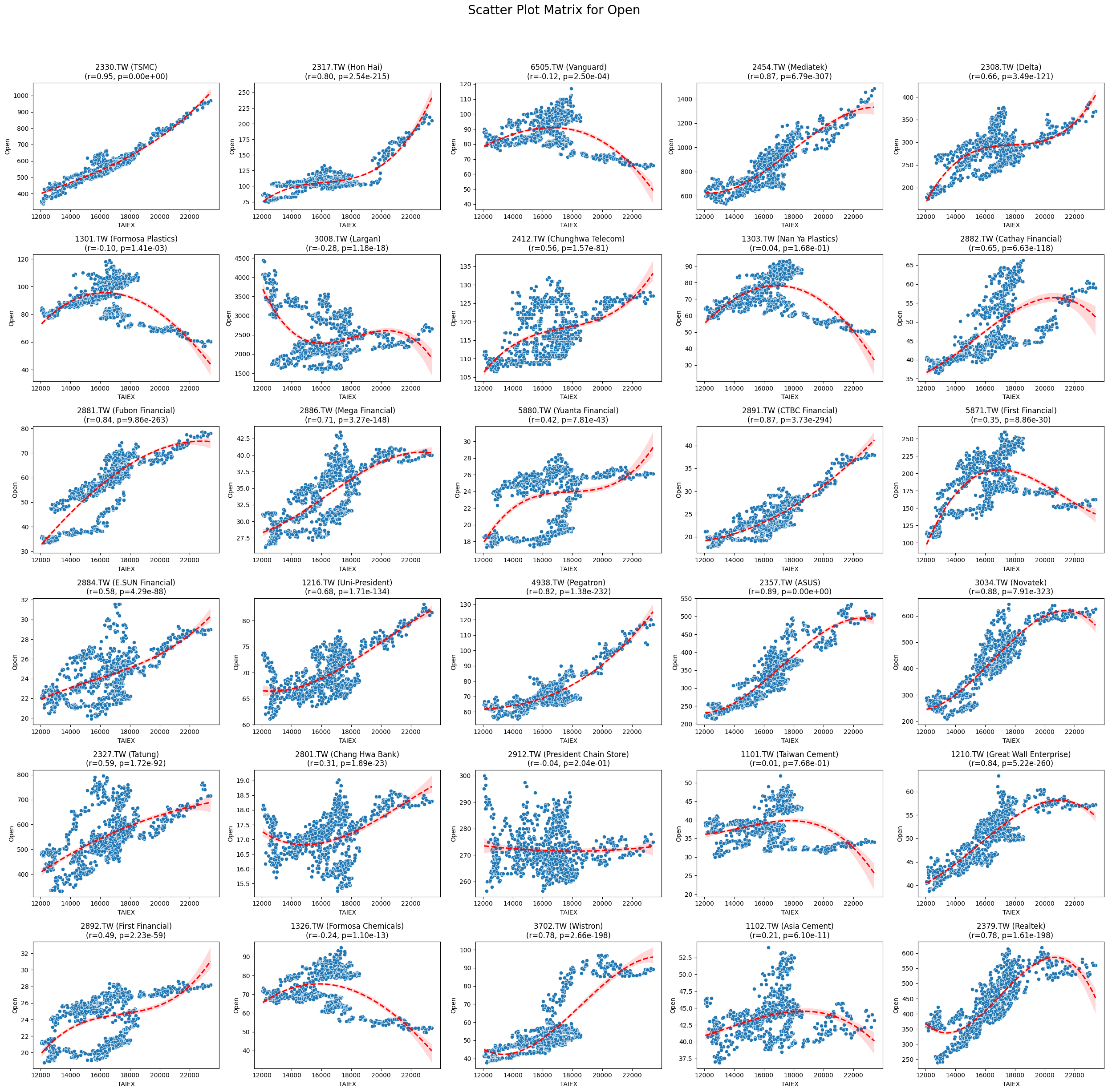
Open 0.022309 5.473519e-05
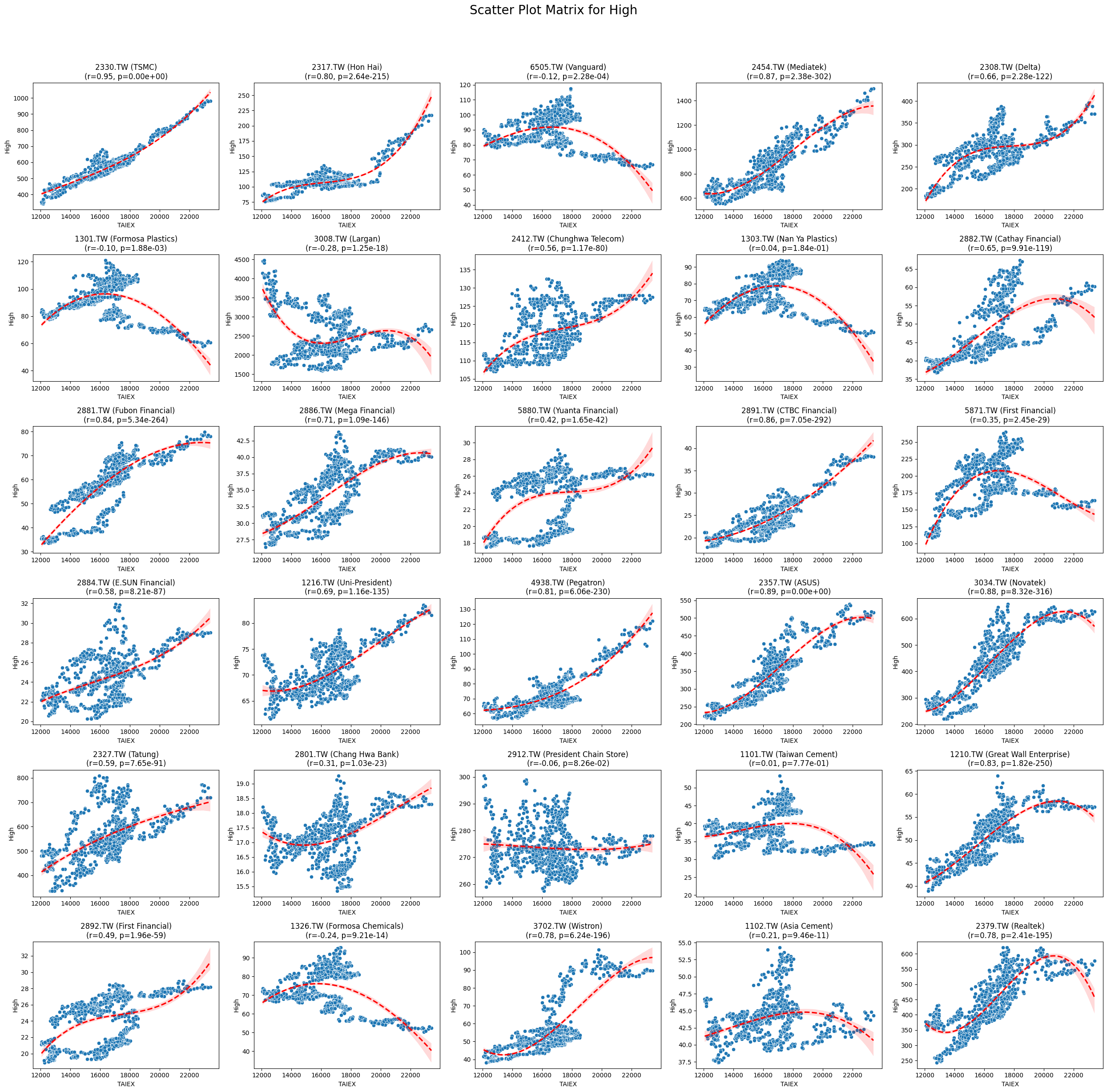
High 0.022106 6.395461e-05
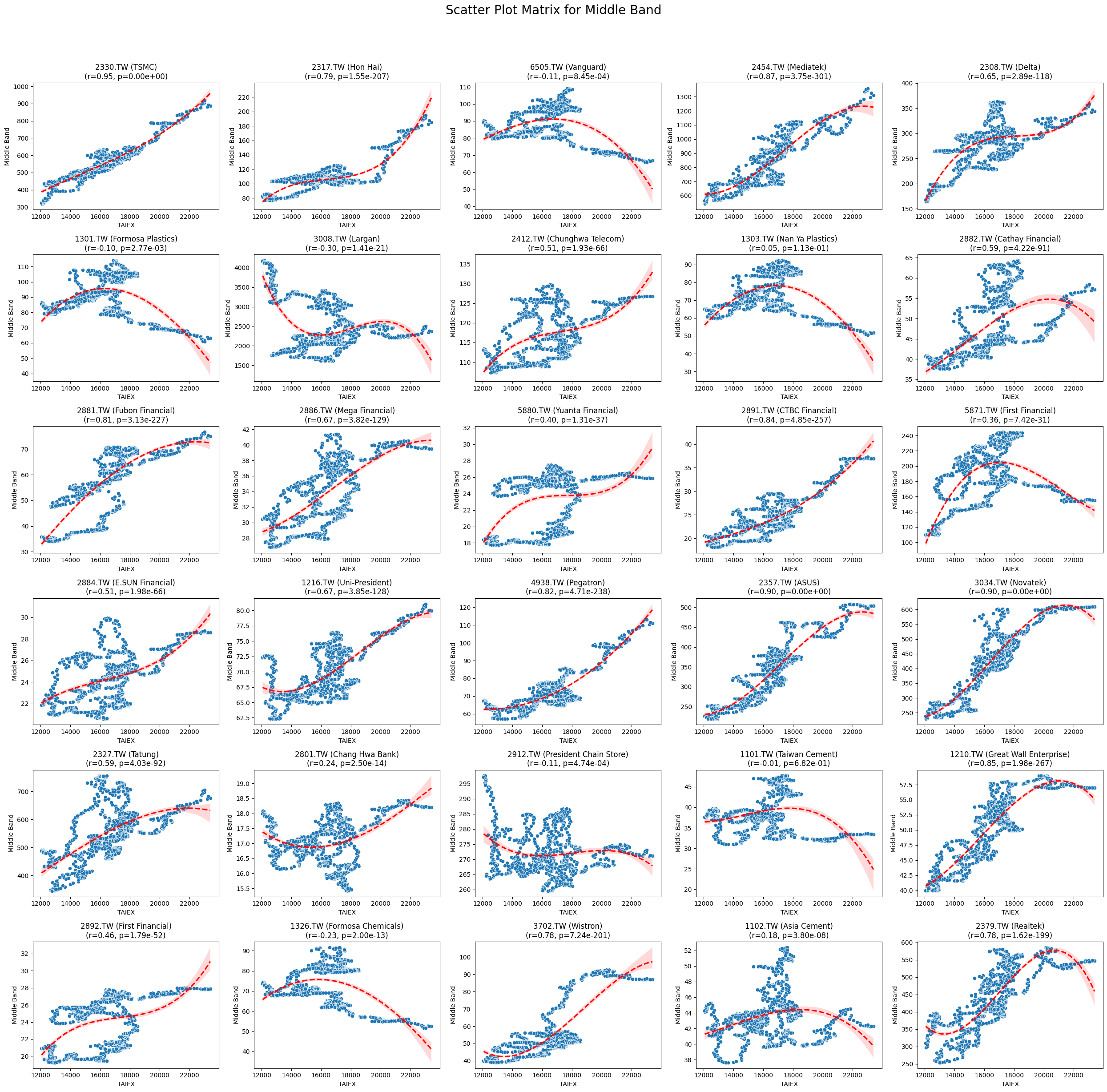
Middle Band 0.021825 9.140844e-05
MA21 0.021806 9.338782e-05
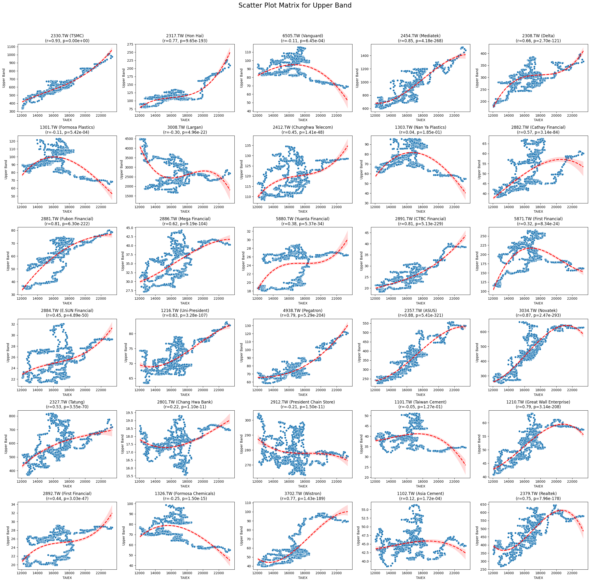
Upper Band 0.018484 9.214753e-04
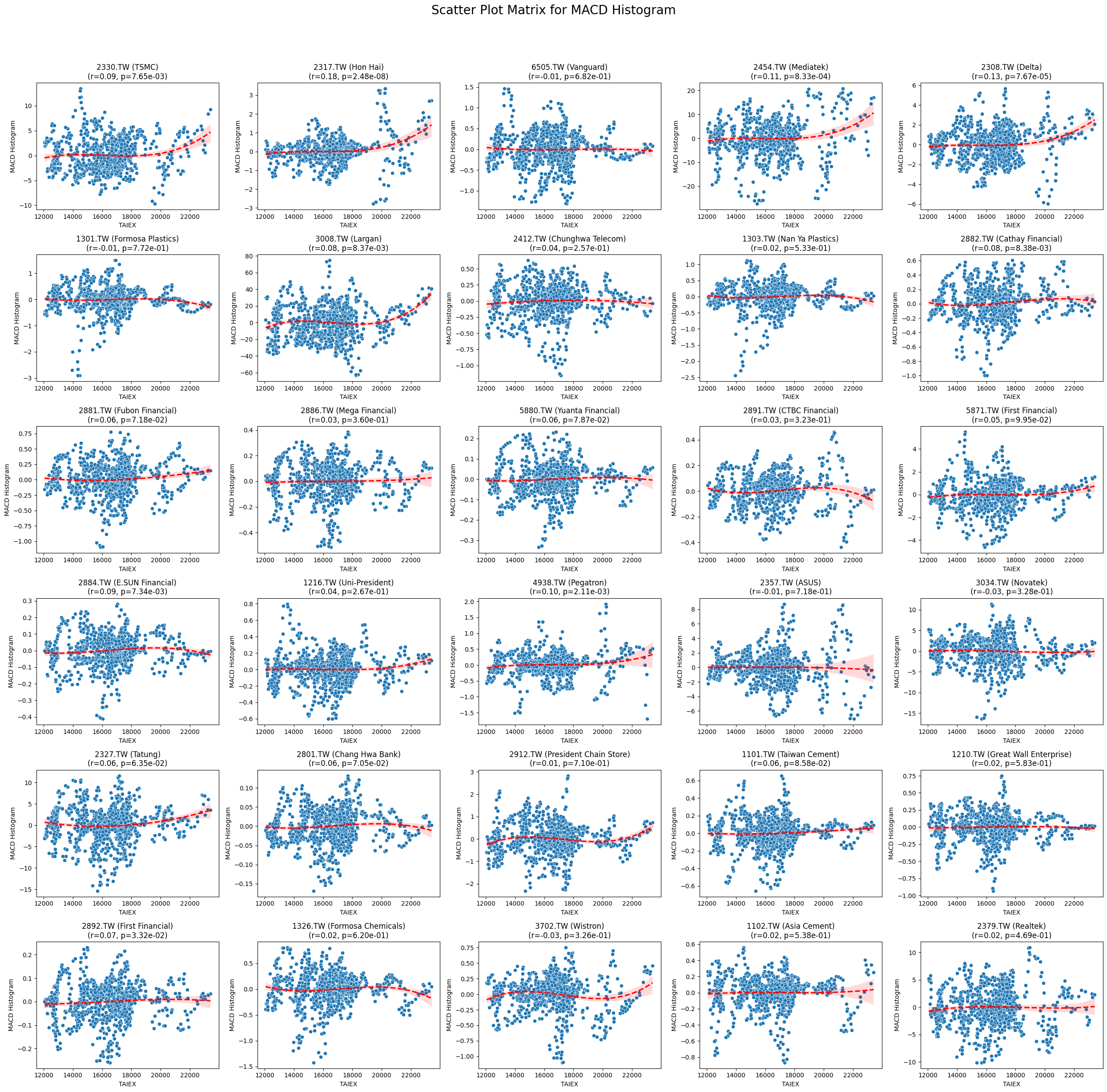
MACD Histogram 0.012701 2.371481e-02
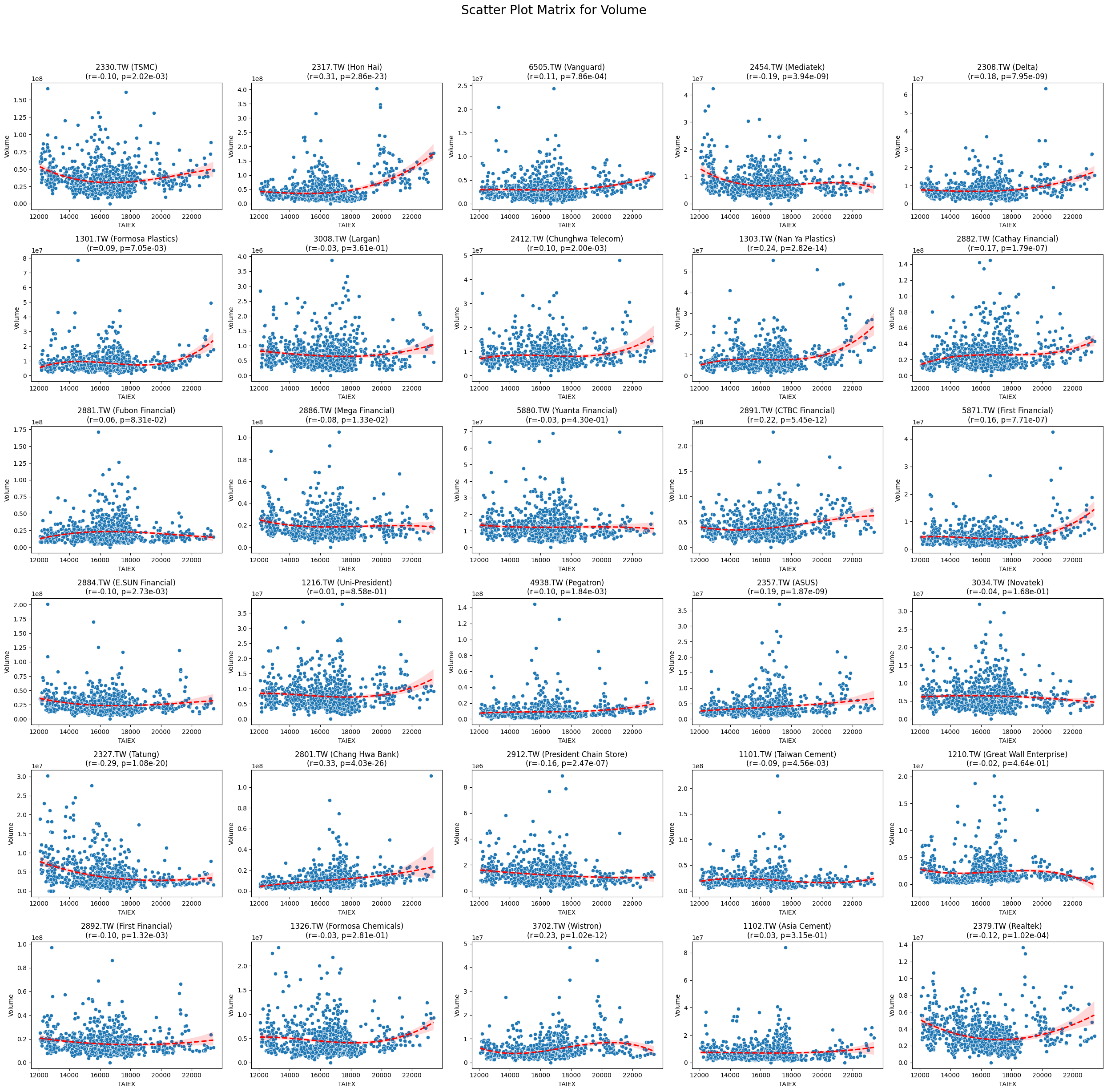
Volume -0.014191 1.028059e-02
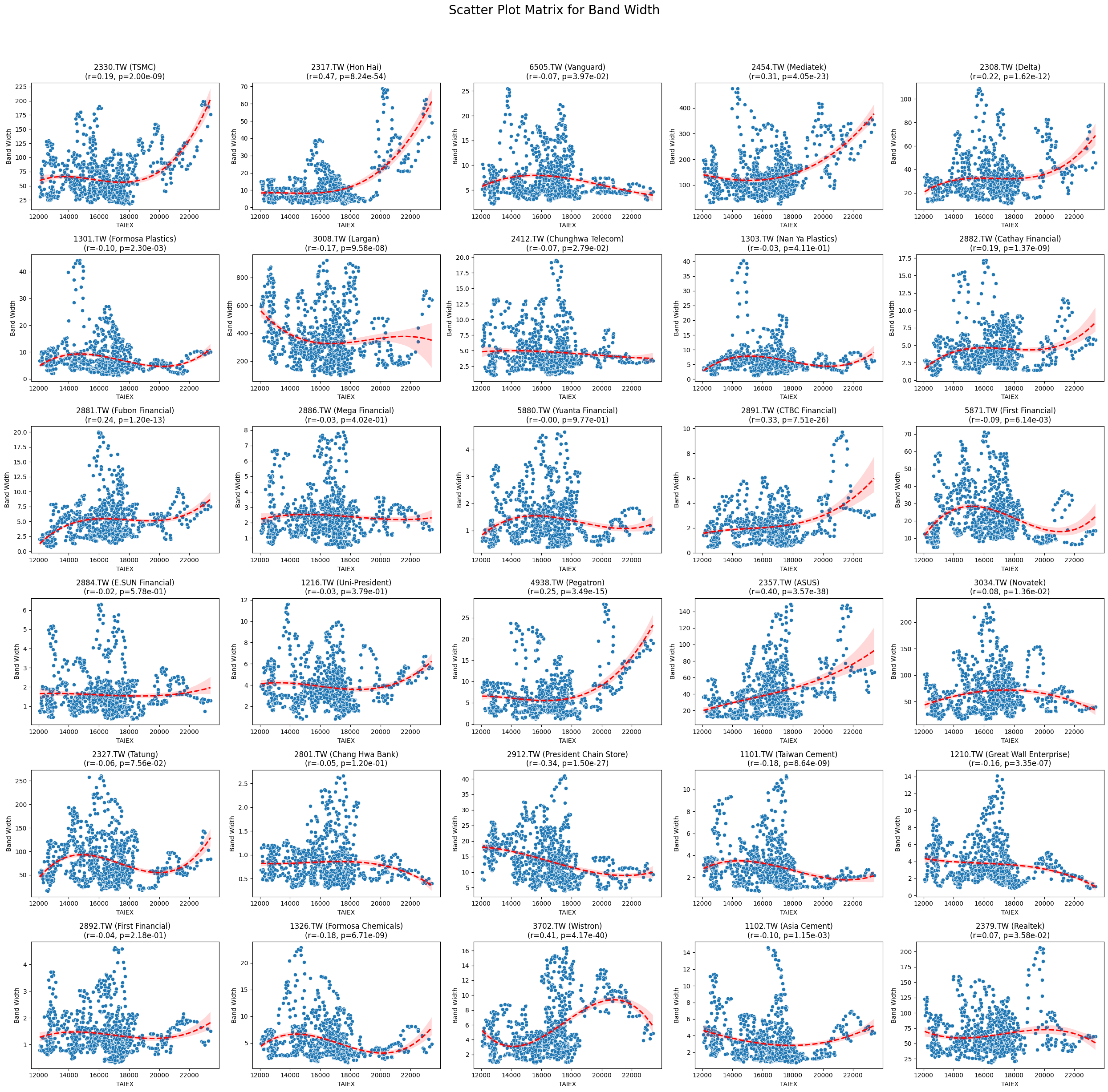
Band Width -0.022150 7.169296e-05
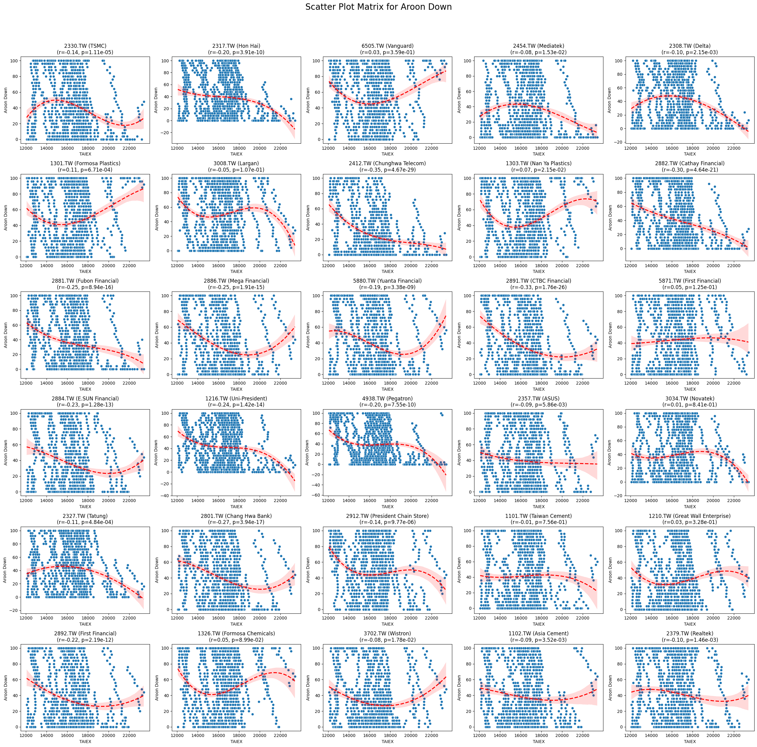
Aroon Down -0.084144 2.690046e-51
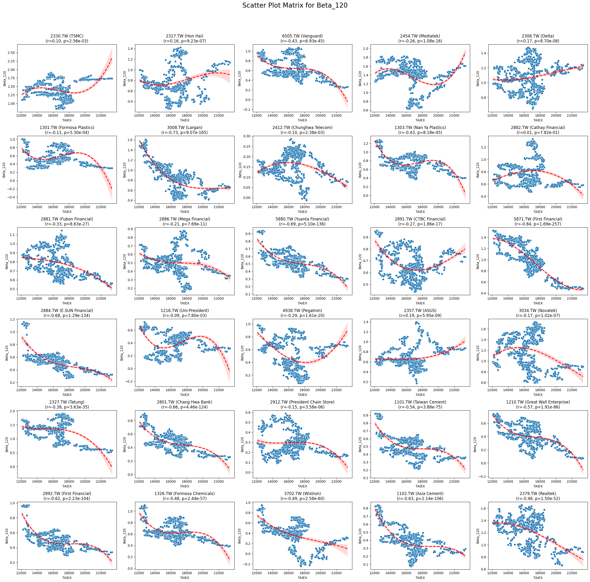
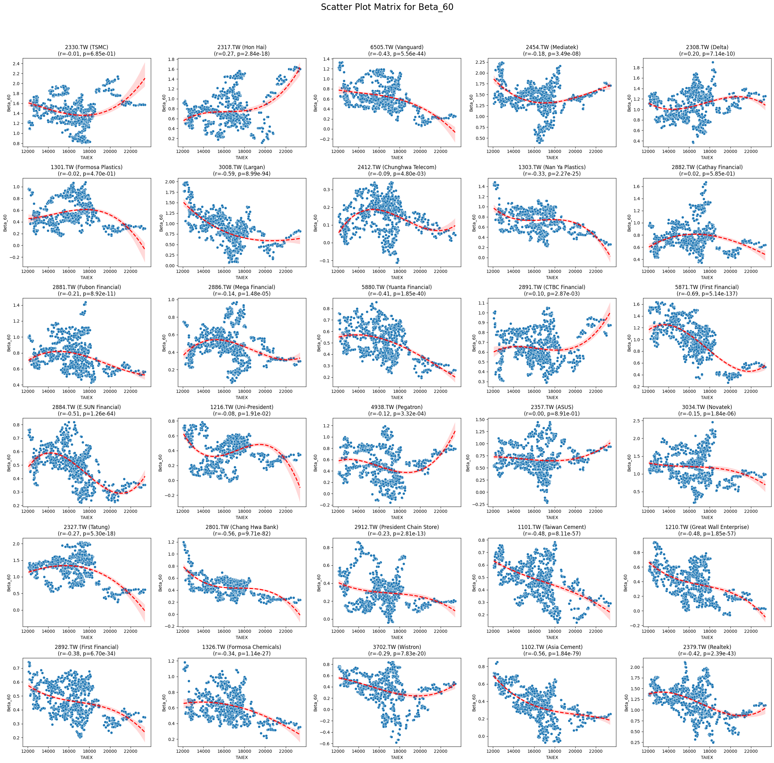
Beta_120 -0.161654 1.405573e-169
Beta_60 -0.183652 1.560559e-232
Stock Pearson Correlation with Close_TAIEX:

Code
import pandas as pd
import numpy as np
import matplotlib.pyplot as plt
import seaborn as sns
from scipy.stats import pearsonr
import statsmodels.api as sm

# Mount Google Drive
from google.colab import drive
drive.mount('/content/drive', force_remount=True)

# Load the data
file_path = '/content/drive/My Drive/MSCI_Taiwan_30_data.csv'
data = pd.read_csv(file_path)

# Convert 'Date' column to datetime
data['Date'] = pd.to_datetime(data['Date'], format='%Y/%m/%d')

# Define the target variable
target_variable = 'Close_TAIEX'

# Function to create scatter plot matrix by variable
def scatter_plot_matrix_by_variable():
    variables = [col for col in data.columns if col not in ['Date', 'ST_Code', 'ST_Name', target_variable]]
    significant_variables = []

    # Identify significant variables
    for variable in variables:
        for stock_code in data['ST_Code'].unique():
            stock_data = data[data['ST_Code'] == stock_code]
            taiex_data = data[['Date', target_variable]].drop_duplicates()
            aligned_data = pd.merge(stock_data, taiex_data, on='Date', suffixes=('', '_TAIEX'))
            aligned_data = aligned_data.replace([np.inf, -np.inf], np.nan).dropna()
            if aligned_data.shape[0] > 0 and variable in aligned_data.columns:
                correlation, p_value = pearsonr(aligned_data[target_variable], aligned_data[variable])
                if p_value <= 0.05:
                    significant_variables.append(variable)
                    break

    significant_variables = list(set(significant_variables))  # Remove duplicates

    # Generate scatter plot matrix for each significant variable
    for variable in significant_variables:
        plt.figure(figsize=(25, 25))
        unique_stock_codes = data['ST_Code'].unique()

        for i, stock_code in enumerate(unique_stock_codes):
            stock_data = data[data['ST_Code'] == stock_code]
            taiex_data = data[['Date', target_variable]].drop_duplicates()
            aligned_data = pd.merge(stock_data, taiex_data, on='Date', suffixes=('', '_TAIEX'))
            aligned_data = aligned_data.replace([np.inf, -np.inf], np.nan).dropna()

            if aligned_data.shape[0] > 0 and variable in aligned_data.columns:
                correlation, p_value = pearsonr(aligned_data[target_variable], aligned_data[variable])
                plt.subplot((len(unique_stock_codes) + 4) // 5, 5, i + 1)
                sns.scatterplot(x=aligned_data[target_variable], y=aligned_data[variable])
                sns.regplot(x=aligned_data[target_variable], y=aligned_data[variable], scatter=False, color='red', ci=95, order=3, line_kws={'linestyle': 'dashed'})
                stock_name = aligned_data['ST_Name'].iloc[0]  # Get the stock name from the first row
                plt.title(f'{stock_code} ({stock_name})\n(r={correlation:.2f}, p={p_value:.2e})')
                plt.xlabel('TAIEX')
                plt.ylabel(variable)

        plt.suptitle(f'Scatter Plot Matrix for {variable}', fontsize=20)
        plt.tight_layout(rect=[0, 0, 1, 0.95])
        plt.savefig(f'/content/drive/My Drive/scatter_plot_matrix_{variable}.png')
        plt.show()

# Generate scatter plot matrix by variable
scatter_plot_matrix_by_variable()