import pandas as pd
import matplotlib.pyplot as plt
import numpy as np
from sklearn.preprocessing import MinMaxScaler
from sklearn.metrics import mean_squared_error
import math
import xgboost as xgb  # 確保導入 XGBoost
from sklearn.model_selection import GridSearchCV
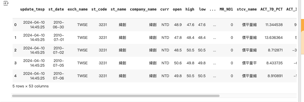
df = pd.read_csv('/content/3231_0614t.csv')
df.head()
# 重置索引提取 'Close' 列
df['st_date'] = pd.to_datetime(df['st_date'])
df2 = df.reset_index()[['st_date', 'close']]
# 建更多特徵
df2['Year'] = df2['st_date'].dt.year
df2['Month'] = df2['st_date'].dt.month
df2['Weekday'] = df2['st_date'].dt.weekday
df2['MA5'] = df2['close'].rolling(window=5).mean()
df2['MA10'] = df2['close'].rolling(window=10).mean()
df2['MA20'] = df2['close'].rolling(window=20).mean()
df2 = df2.dropna()
# 創建數據集
train_size = int(len(df2_scaled) * 0.65)
test_size = len(df2_scaled) - train_size
train_data, test_data = df2_scaled[0:train_size, :], df2_scaled[train_size:len(df2_scaled), :]

# 數據集
def create_dataset(dataset, time_step=1):
    dataX, dataY = [], []
    for i in range(len(dataset) - time_step - 1):
        a = dataset[i:(i + time_step), :]
        dataX.append(a)
        dataY.append(dataset[i + time_step, 0])  # 預測 'close' 列
    return np.array(dataX), np.array(dataY)

time_step = 100
X_train, Y_train = create_dataset(train_data, time_step)
X_test, Y_test = create_dataset(test_data, time_step)

# XGBoost的格式
X_train = X_train.reshape(X_train.shape[0], -1)
X_test = X_test.reshape(X_test.shape[0], -1)

# XGBoost模型和参數
xg_reg = xgb.XGBRegressor(objective='reg:squarederror', missing=np.nan)

param_grid = {
    'colsample_bytree': [0.3, 0.5, 0.7],
    'learning_rate': [0.01, 0.1, 0.2],
    'max_depth': [3, 5, 7],
    'n_estimators': [100, 200, 300],
    'subsample': [0.6, 0.8, 1.0],
    'gamma': [0, 0.1, 0.2]
}
# 進進網格搜索
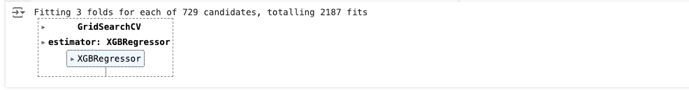
grid_search = GridSearchCV(estimator=xg_reg, param_grid=param_grid, scoring='neg_mean_squared_error', cv=3, verbose=1)
grid_search.fit(X_train, Y_train)
# 穫取最佳参数
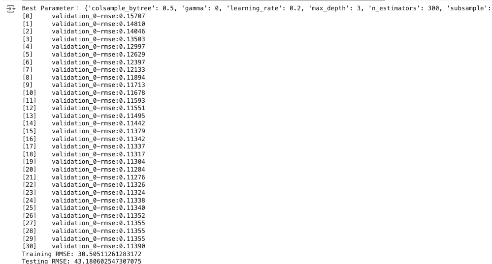
best_params = grid_search.best_params_
print("Best Parameter:", best_params)
# 使用最佳参数訓練模型
xg_reg_best = xgb.XGBRegressor(**best_params, early_stopping_rounds=10, eval_metric='rmse')
xg_reg_best.fit(X_train, Y_train, eval_set=[(X_test, Y_test)], verbose=True)
# 預測
train_predict = xg_reg_best.predict(X_train)
test_predict = xg_reg_best.predict(X_test)
# 反歸一化預測結果
train_predict_inverse = scaler.inverse_transform(train_data[time_step:len(train_predict) + time_step, :]) # Pass the original training data with all features
test_predict_inverse = scaler.inverse_transform(test_data[time_step:len(test_predict) + time_step, :]) # Pass the original testing data with all features
# Extract the 'close' column for RMSE calculation
train_predict = train_predict_inverse[:, 0]
test_predict = test_predict_inverse[:, 0]
# 計算RMSE
rmse_train = math.sqrt(mean_squared_error(Y_train, train_predict))
print("Training RMSE:", rmse_train)
rmse_test = math.sqrt(mean_squared_error(Y_test, test_predict))
print("Testing RMSE:", rmse_test)
# 繪制預測結果
look_back = time_step
trainPredictPlot = np.empty_like(df2_scaled[:, 0])
trainPredictPlot[:] = np.nan
trainPredictPlot[look_back:len(train_predict) + look_back] = train_predict
testPredictPlot = np.empty_like(df2_scaled[:, 0])
testPredictPlot[:] = np.nan
testPredictPlot[len(train_predict) + (look_back * 2) + 1:len(df2_scaled) - 1] = test_predict
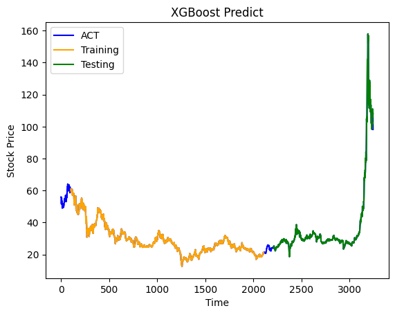
plt.plot(scaler.inverse_transform(df2_scaled)[:, 0], color='blue', label='ACT')
plt.plot(trainPredictPlot, color='orange', label='Training')
plt.plot(testPredictPlot, color='green', label='Testing')
plt.title('XGBoost Predict')
plt.xlabel('Time')
plt.ylabel('Stock Price')
plt.legend()
plt.show()