SVM.dft1.TAIEX.POC.0628

from google.colab import drive
drive.mount('/content/drive')

!pip install yfinance scikit-learn matplotlib statsmodels ta
import yfinance as yf
import pandas as pd
import numpy as np
import matplotlib.pyplot as plt
from sklearn.preprocessing import MinMaxScaler
from sklearn.svm import SVR
from sklearn.decomposition import PCA
from sklearn.metrics import mean_squared_error, mean_absolute_error, roc_curve, roc_auc_score
from sklearn.model_selection import GridSearchCV
import statsmodels.api as sm
import ta

# 計算 Chande Momentum Oscillator (CMO)
def calculate_cmo(data, window):
    delta = data.diff()
    up = delta.where(delta > 0, 0.0)
    down = -delta.where(delta < 0, 0.0)
    sum_up = up.rolling(window=window).sum()
    sum_down = down.rolling(window=window).sum()
    cmo = 100 * (sum_up - sum_down) / (sum_up + sum_down)
    return cmo

# 下載數據
tickers = ['2330.TW', '2454.TW', '2317.TW', '2412.TW', '1303.TW', '2882.TW', 
           '3008.TW', '2308.TW', '1402.TW', '1216.TW', '2881.TW', '2891.TW', 
           '2382.TW', '2409.TW', '1802.TW', '1101.TW', '3045.TW', '2324.TW', 
           '2105.TW', '2880.TW', '2887.TW', '2885.TW', '4904.TW', '2603.TW', 
           '2884.TW', '2886.TW', '2357.TW', '2344.TW', '4938.TW', '2888.TW', '^TWII']
data = yf.download(tickers, start="2021-01-01", end="2024-06-28")
adj_close = data['Adj Close']
high = data['High']
low = data['Low']

# 計算技術指標
features = pd.DataFrame(index=adj_close.index)
twii_returns = adj_close['^TWII'].pct_change()
for ticker in tickers[:-1]:  # 不包括 '^TWII'
    stock_returns = adj_close[ticker].pct_change()
    cov_matrix = stock_returns.rolling(window=120).cov(twii_returns)
    var = twii_returns.rolling(window=120).var()
    features[f'{ticker}_beta'] = cov_matrix / var
    features[f'{ticker}_MA7'] = adj_close[ticker].rolling(window=7).mean()
    features[f'{ticker}_RSI14'] = ta.momentum.RSIIndicator(close=adj_close[ticker], window=14).rsi()
    features[f'{ticker}_Bollinger_upper'] = ta.volatility.BollingerBands(close=adj_close[ticker], window=20, window_dev=2).bollinger_hband()
    features[f'{ticker}_Bollinger_lower'] = ta.volatility.BollingerBands(close=adj_close[ticker], window=20, window_dev=2).bollinger_lband()
    features[f'{ticker}_Aroon_up'] = ta.trend.AroonIndicator(high=high[ticker], low=low[ticker], window=25).aroon_up()
    features[f'{ticker}_Aroon_down'] = ta.trend.AroonIndicator(high=high[ticker], low=low[ticker], window=25).aroon_down()
    features[f'{ticker}_CCI'] = ta.trend.CCIIndicator(high=high[ticker], low=low[ticker], close=adj_close[ticker], window=20).cci()
    features[f'{ticker}_CMO'] = calculate_cmo(adj_close[ticker], window=14)
    features[f'{ticker}_WILLR'] = ta.momentum.WilliamsRIndicator(high=high[ticker], low=low[ticker], close=adj_close[ticker], lbp=14).williams_r()

# 移除 P 值大於 0.05 的變數
X = features.dropna()
y = adj_close['^TWII'].loc[X.index.to_list()]

# 標準化
scaler = MinMaxScaler()
X_scaled = scaler.fit_transform(X)

# PCA 降維
pca = PCA(n_components=0.95)  # 保留 95% 的方差
X_pca = pca.fit_transform(X_scaled)

# OLS 回歸
X_pca_const = sm.add_constant(X_pca)
model = sm.OLS(y, X_pca_const).fit()
print(model.summary())

# 分割數據集
train_size = 0.8
train_index = int(len(X_pca) * train_size)
X_train_pca, X_test_pca = X_pca[:train_index], X_pca[train_index:]
y_train, y_test = y[:train_index], y[train_index:]

# 支持向量機回歸
param_grid = {
    'C': [0.1, 1, 10, 100],
    'gamma': [1, 0.1, 0.01, 0.001],
    'epsilon': [0.1, 0.2, 0.5, 0.3],
    'kernel': ['rbf']
}
grid_search = GridSearchCV(SVR(), param_grid, refit=True, cv=5, n_jobs=-1)
grid_search.fit(X_train_pca, y_train)

# 預測
train_predict = grid_search.predict(X_train_pca)
test_predict = grid_search.predict(X_test_pca)

# 限制每日最大漲跌幅為 10%
def limit_change(predictions, previous_value, max_change=0.1):
    limited_predictions = []
    for pred in predictions:
        change = (pred - previous_value) / previous_value
        if change > max_change:
            pred = previous_value * (1 + max_change)
        elif change < -max_change:
            pred = previous_value * (1 - max_change)
        limited_predictions.append(pred)
        previous_value = pred
    return np.array(limited_predictions)

# 應用漲跌幅限制
train_predict = limit_change(train_predict, y_train.iloc[0])
test_predict = limit_change(test_predict, y_test.iloc[0])

# 計算 MSE 和 MAE
train_mse = mean_squared_error(y_train, train_predict)
test_mse = mean_squared_error(y_test, test_predict)
train_mae = mean_absolute_error(y_train, train_predict)
test_mae = mean_absolute_error(y_test, test_predict)

print(f"Training MSE: {train_mse:.4f}")
print(f"Testing MSE: {test_mse:.4f}")
print(f"Training MAE: {train_mae:.4f}")
print(f"Testing MAE: {test_mae:.4f}")

# 二元分類
threshold = np.median(y_test)  # 設定閾值為測試數據的中位數
y_test_class = (y_test > threshold).astype(int)
test_predict_class = (test_predict > threshold).astype(int)

# 確保有兩個類別
if len(np.unique(y_test_class)) > 1:
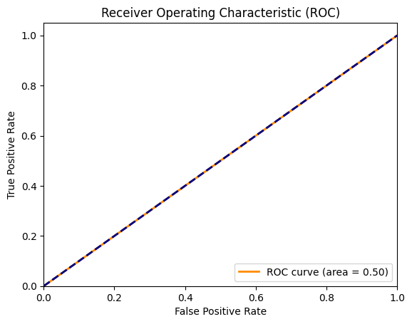
    # 計算 ROC 曲線和 AUC 值
    fpr, tpr, _ = roc_curve(y_test_class, test_predict_class)
    roc_auc = roc_auc_score(y_test_class, test_predict_class)

    # 繪製 ROC 曲線
    plt.figure()
    plt.plot(fpr, tpr, color='darkorange', lw=2, label='ROC curve (area = %0.2f)' % roc_auc)
    plt.plot([0, 1], [0, 1], color='navy', lw=2, linestyle='--')
    plt.xlim([0.0, 1.0])
    plt.ylim([0.0, 1.05])
    plt.xlabel('False Positive Rate')
    plt.ylabel('True Positive Rate')
    plt.title('Receiver Operating Characteristic (ROC)')
    plt.legend(loc="lower right")
    plt.show()
else:
    print("ROC AUC score is not defined as there is only one class present in y_test_class.")

# 繪製整個數據集的走勢圖
plt.figure(figsize=(14, 7))
plt.plot(y_train.index, y_train, color='blue', label='ACTUAL')
plt.plot(y_train.index, train_predict, color='orange', label='Training')
plt.plot(y_test.index, y_test, color='blue')
plt.plot(y_test.index, test_predict, color='red', label='Prediction')
plt.legend()  # 確保圖例顯示
plt.xlabel('Date')
plt.ylabel('TAIEX')
plt.title('TAIEX Prediction')
plt.grid(True)
plt.show()

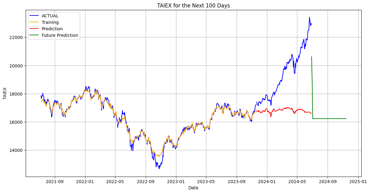
# 預測未來 100 天的走勢
future_dates = pd.date_range(start=y_test.index[-1], periods=101, freq='B')[1:]
future_features = X_test_pca[-1:].copy()
future_predictions = []

for i in range(100):
    next_day = grid_search.best_estimator_.predict(future_features.reshape(1, -1))[0]
    future_predictions.append(next_day)
    next_day_features = np.array([next_day] * future_features.shape[1]).reshape(1, -1)
    future_features = np.append(future_features[1:], next_day_features, axis=0)

# 應用漲跌幅限制
future_predictions = limit_change(future_predictions, y_test.iloc[-1])

# 顯示未來 100 天的預測結果
plt.figure(figsize=(14, 7))
plt.plot(y_train.index, y_train, color='blue', label='ACTUAL')
plt.plot(y_train.index, train_predict, color='orange', label='Training')
plt.plot(y_test.index, y_test, color='blue')
plt.plot(y_test.index, test_predict, color='red', label='Prediction')
plt.plot(future_dates, future_predictions, color='green', label='Future Prediction')
plt.legend()  # 確保圖例顯示
plt.xlabel('Date')
plt.ylabel('TAIEX')
plt.title('TAIEX for the Next 100 Days')
plt.grid(True)
plt.show()

  基本變數
Adj Close: 股票的調整收盤價
High: 股票的最高價
Low: 股票的最低價
計算出的技術指標變數
beta: 股票的 Beta 值（與台灣加權指數的協方差除以台灣加權指數的方差）
MA7: 7 天移動平均線
RSI14: 14 天相對強弱指數
Bollinger_upper: 布林帶上軌
Bollinger_lower: 布林帶下軌
Aroon_up: Aroon 指標中的上升線
Aroon_down: Aroon 指標中的下降線
CCI: 商品通道指標
CMO: Chande 動量擺動指標
WILLR: 威廉指數
使用的技術指標變數（每個股票的技術指標變數前綴為股票代碼）
例如：

2330.TW_beta
2330.TW_MA7
2330.TW_RSI14
2330.TW_Bollinger_upper
2330.TW_Bollinger_lower
2330.TW_Aroon_up
2330.TW_Aroon_down
2330.TW_CCI
2330.TW_CMO
2330.TW_WILLR


同樣地，其他股票的變數名稱也遵循相同的命名方式，例如 2454.TW_beta、2454.TW_MA7 等等。

目標變數
y: 台灣加權指數 (^TWII) 的調整收盤價。
PCA 降維
PCA 將高維度的特徵空間降維到保留 95% 方差的低維空間。具體的變數數量取決於原始特徵的數量和數據的內在結構。

OLS 回歸中的變數
在進行 OLS 回歸時，我們會對經過標準化和 PCA 降維後的變數進行回歸。這些變數經過降維後變成了主成分變數（Principal Components）。

具體到這個代碼中，我們使用的變數總數（原始特徵）會很多，但經過 PCA 降維後實際使用的變數數量會減少，保留了最重要的幾個主成分。

變數摘要

1. 基本變數：Adj Close、High、Low
2. 技術指標變數：beta、MA7、RSI14、Bollinger_upper、Bollinger_lower、Aroon_up、Aroon_down、CCI、CMO、WILLR
3. 使用的技術指標變數（每個股票的技術指標變數前綴為股票代碼）：
   • 2330.TW_beta、2330.TW_MA7、2330.TW_RSI14、2330.TW_Bollinger_upper、2330.TW_Bollinger_lower、2330.TW_Aroon_up、2330.TW_Aroon_down、2330.TW_CCI、2330.TW_CMO、2330.TW_WILLR
   • 其他股票變數名稱也遵循相同的命名方式
4. 目標變數：台灣加權指數 (^TWII) 的調整收盤價 adj_close['^TWII']
5. PCA 降維後的主成分變數：使用 PCA 降維後的主成分變數

這些變數經過降維後成為主成分變數，並應用於 OLS 回歸和支持向量機回歸中。