# Missing values analysis
missing_values = data.isnull().sum()
print("Missing Values Analysis:")
print(missing_values)
Missing Values Analysis:
Date                 0
ST_Code              0
ST_Name              0
Open                 0
High                 0
Low                  0
Close_MSCI           0
Adj_Close            0
Volume               0
MA7                180
MA21               600
MA50              1470
MA100             2970
Middle Band        570
Upper Band         570
Lower Band         570
Band Width         570
Aroon Up           750
Aroon Down         750
CCI20              570
CMO14              390
MACD Line          750
Signal Line        990
MACD Histogram     990
RSI7               180
RSI14              390
RSI21              600
%K                 390
%D                 450
WILLR14            390
Market Return       30
Stock Return        30
Beta_60           1800
Beta_120          3600
Close_TAIEX          0
OBV                  0
dtype: int64
- 首先排除了非數值型數據
- 然後對數值型數據進行均值填補
- 並重新進行缺失值分析和描述性統計分析。
- 接著重新繪製了每個變數的 Box Plot Matrix Map。
import pandas as pd

# 加載數據
file_path = '/content/drive/My Drive/MSCI_Taiwan_30_data_with_OBV.csv'
data = pd.read_csv(file_path)

# 顯示缺失值分析結果
missing_values = data.isnull().sum()
print("Missing Values Analysis:")
print(missing_values)

# 排除非數值列
numeric_data = data.select_dtypes(include=[float, int])

# 填補缺失值,使用列的均值
data_filled = numeric_data.fillna(numeric_data.mean())

# 顯示填補後的缺失值分析結果
missing_values_filled = data_filled.isnull().sum()
print("Missing Values Analysis After Filling:")
print(missing_values_filled)

# 確認填補後數據集是否仍有缺失值
assert missing_values_filled.sum() == 0, "There are still missing values after filling!"
print("All missing values have been successfully filled.")

# 描述性統計
descriptive_stats_filled = data_filled.describe()
print("Descriptive Statistics After Filling Missing Values:")
print(descriptive_stats_filled)
[1]
26 秒
from google.colab import drive
drive.mount('/content/drive')
Mounted at /content/drive
[10]
12 秒
import pandas as pd
import matplotlib.pyplot as plt
import seaborn as sns
from scipy import stats
# Load the data
file_path = '/content/drive/My Drive/MSCI_Taiwan_30_data_with_OBV.csv'
data = pd.read_csv(file_path)
# Descriptive statistics
descriptive_stats = data.describe()
print("Descriptive Statistics:")
print(descriptive_stats)
# Plot histograms
data.hist(bins=50, figsize=(20, 15))
plt.suptitle('Histograms of Variables')
plt.show()
[11]
15 分鐘
# Sample data
sampled_data = data.sample(n=1000, random_state=42)
# Plot pairwise relationships
sns.pairplot(sampled_data)
plt.suptitle('Scatter Plot of Variables', y=1.02)
plt.show()
[18]
4 秒
sns.heatmap(correlation_matrix, annot=True, cmap='coolwarm', annot_kws={"size": 6.5})
plt.title('Correlation Heatmap')
plt.show()
[21]
0 秒
# Normality test
print("Normality Test:")
for column in numeric_data.columns:
stat, p = stats.shapiro(numeric_data[column].dropna())
print(f'{column}: Statistics={stat}, p={p}')
Normality Test:
Open: Statistics=0.44388264417648315, p=0.0
High: Statistics=0.44386327266693115, p=0.0
Low: Statistics=0.44448310136795044, p=0.0
Close_MSCI: Statistics=0.44464701414108276, p=0.0
Adj_Close: Statistics=0.44800859689712524, p=0.0
Volume: Statistics=0.616114616394043, p=0.0
MA7: Statistics=0.4454984664916992, p=0.0
MA21: Statistics=0.4475475549697876, p=0.0
MA50: Statistics=0.4513601064682007, p=0.0
MA100: Statistics=0.45628875494003296, p=0.0
Middle Band: Statistics=0.44740188121795654, p=0.0
Upper Band: Statistics=0.44556015729904175, p=0.0
Lower Band: Statistics=0.44893014430999756, p=0.0
Band Width: Statistics=0.37196314334869385, p=0.0
Aroon Up: Statistics=0.8953447341918945, p=0.0
Aroon Down: Statistics=0.8862640261650085, p=0.0
CCI20: Statistics=0.9935651421546936, p=1.4978255776941871e-34
CMO14: Statistics=0.9970583319664001, p=4.02672471348255e-24
MACD Line: Statistics=0.4291476607322693, p=0.0
Signal Line: Statistics=0.4337118864059448, p=0.0
MACD Histogram: Statistics=0.4151105284690857, p=0.0
RSI7: Statistics=0.9972341656684875, p=1.9062553984236165e-23
RSI14: Statistics=0.9991347789764404, p=1.0700896765913903e-11
RSI21: Statistics=0.998984158039093, p=5.296772677583494e-13
%K: Statistics=0.9418363571166992, p=0.0
%D: Statistics=0.9411165714263916, p=0.0
WILLR14: Statistics=0.9418363571166992, p=0.0
Market Return: Statistics=0.9587656259536743, p=0.0
Stock Return: Statistics=0.9099488854408264, p=0.0
Beta_60: Statistics=0.9558936357498169, p=0.0
Beta_120: Statistics=0.9457791447639465, p=0.0
Close_TAIEX: Statistics=0.9737288951873779, p=0.0
OBV: Statistics=0.9423521161079407, p=0.0
[25]
18 秒
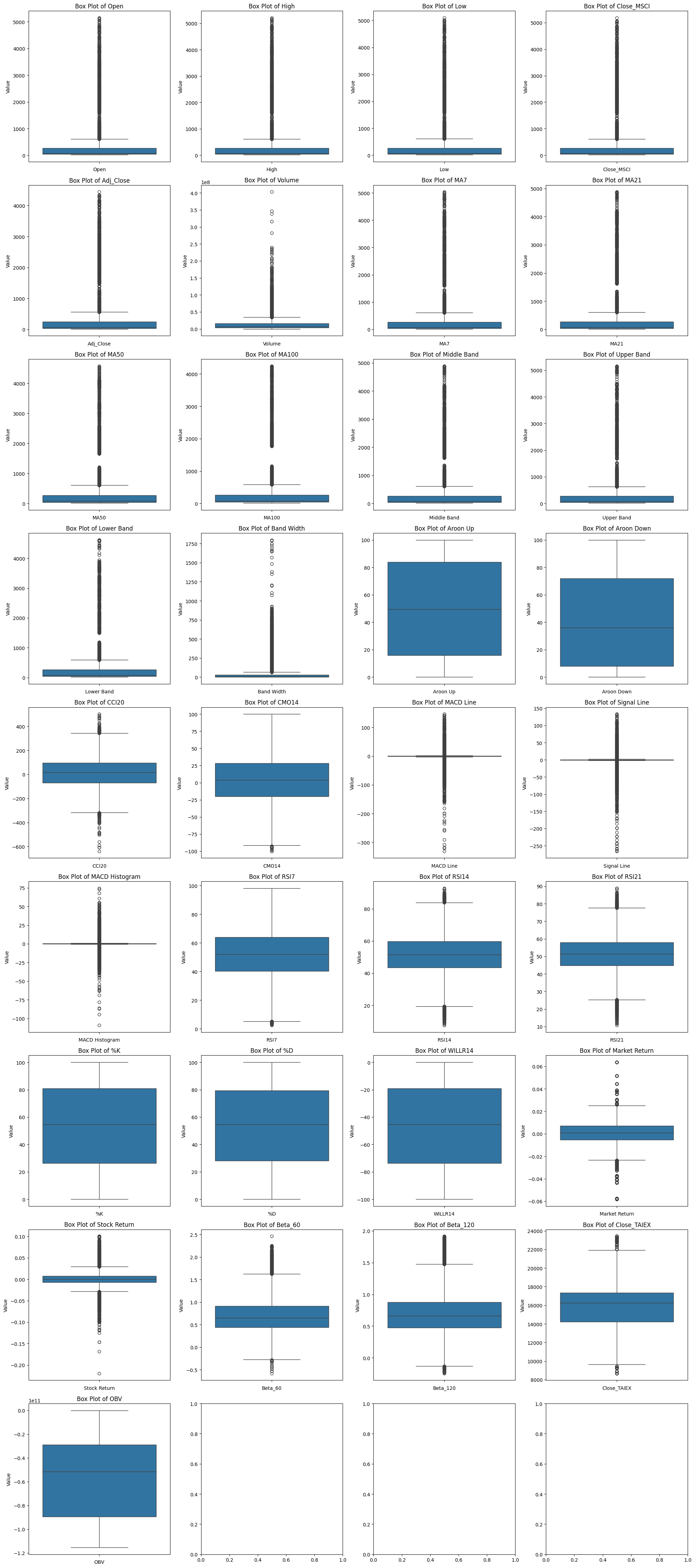
import math
import pandas as pd
import matplotlib.pyplot as plt
import seaborn as sns
# 加載數據
file_path = '/content/drive/My Drive/MSCI_Taiwan_30_data_with_OBV.csv'
data = pd.read_csv(file_path)
# 排除非數值列
numeric_data = data.drop(columns=['Date', 'ST_Code', 'ST_Name'])
# 獲取變數列表
variables = numeric_data.columns
# 設置圖表大小
num_vars = len(variables)
num_cols = 4
num_rows = math.ceil(num_vars / num_cols)
fig, axes = plt.subplots(num_rows, num_cols, figsize=(20, num_rows * 5))
# 繪製每個變數的 Box Plot
for i, var in enumerate(variables):
row = i // num_cols
col = i % num_cols
sns.boxplot(data=numeric_data[var], ax=axes[row, col])
axes[row, col].set_title(f'Box Plot of {var}')
axes[row, col].set_xlabel(var)
axes[row, col].set_ylabel('Value')
# 調整佈局
plt.tight_layout()
plt.show()
[29]
0 秒
import pandas as pd
# 加載數據
file_path = '/content/drive/My Drive/MSCI_Taiwan_30_data_with_OBV.csv'
data = pd.read_csv(file_path)
# 顯示缺失值分析結果
missing_values = data.isnull().sum()
print("Missing Values Analysis:")
print(missing_values)
Missing Values Analysis:
Date 0
ST_Code 0
ST_Name 0
Open 0
High 0
Low 0
Close_MSCI 0
Adj_Close 0
Volume 0
MA7 180
MA21 600
MA50 1470
MA100 2970
Middle Band 570
Upper Band 570
Lower Band 570
Band Width 570
Aroon Up 750
Aroon Down 750
CCI20 570
CMO14 390
MACD Line 750
Signal Line 990
MACD Histogram 990
RSI7 180
RSI14 390
RSI21 600
%K 390
%D 450
WILLR14 390
Market Return 30
Stock Return 30
Beta_60 1800
Beta_120 3600
Close_TAIEX 0
OBV 0
dtype: int64
[30]
2 秒
# 填補缺失值,使用列的均值
data_filled = data.fillna(data.mean())
# 顯示填補後的缺失值分析結果
missing_values_filled = data_filled.isnull().sum()
print("Missing Values Analysis After Filling:")
print(missing_values_filled)
後續步驟:
[31]
1 秒
import pandas as pd
# 加載數據
file_path = '/content/drive/My Drive/MSCI_Taiwan_30_data_with_OBV.csv'
data = pd.read_csv(file_path)
# 顯示缺失值分析結果
missing_values = data.isnull().sum()
print("Missing Values Analysis:")
print(missing_values)
…
Missing Values Analysis:
Date 0
ST_Code 0
ST_Name 0
Open 0
High 0
Low 0
Close_MSCI 0
Adj_Close 0
Volume 0
MA7 180
MA21 600
MA50 1470
MA100 2970
Middle Band 570
Upper Band 570
Lower Band 570
Band Width 570
Aroon Up 750
Aroon Down 750
CCI20 570
CMO14 390
MACD Line 750
Signal Line 990
MACD Histogram 990
RSI7 180
RSI14 390
RSI21 600
%K 390
%D 450
WILLR14 390
Market Return 30
Stock Return 30
Beta_60 1800
Beta_120 3600
Close_TAIEX 0
OBV 0
dtype: int64
Missing Values Analysis After Filling:
Open 0
High 0
Low 0
Close_MSCI 0
Adj_Close 0
Volume 0
MA7 0
MA21 0
MA50 0
MA100 0
Middle Band 0
Upper Band 0
Lower Band 0
Band Width 0
Aroon Up 0
Aroon Down 0
CCI20 0
CMO14 0
MACD Line 0
Signal Line 0
MACD Histogram 0
RSI7 0
RSI14 0
RSI21 0
%K 0
%D 0
WILLR14 0
Market Return 0
Stock Return 0
Beta_60 0
Beta_120 0
Close_TAIEX 0
OBV 0
dtype: int64
All missing values have been successfully filled.
Descriptive Statistics After Filling Missing Values:
Open High Low Close_MSCI Adj_Close \
count 32700.000000 32700.000000 32700.000000 32700.000000 32700.000000
mean 250.214867 253.012017 247.112520 249.812194 227.177200
std 512.800070 518.951093 505.316701 511.027804 460.886560
min 14.345764 14.653801 13.949715 14.125737 12.343324
25% 40.170254 40.400002 39.900002 40.146721 36.394313
50% 75.599998 76.350002 75.000000 75.750000 70.308552
75% 269.000000 271.000000 267.500000 269.500000 245.990616
max 5150.000000 5210.000000 5095.000000 5180.000000 4442.363770
Volume MA7 MA21 MA50 MA100 \
count 3.270000e+04 32700.000000 32700.000000 32700.000000 32700.000000
mean 1.272284e+07 249.524745 248.895559 247.962300 247.195609
std 1.695529e+07 508.009952 501.046905 487.944386 469.043215
min 0.000000e+00 15.081283 15.427423 15.700038 15.818984
25% 3.443974e+06 40.276786 40.652381 41.666417 43.076875
50% 7.088050e+06 76.400000 77.657143 80.338000 85.189000
75% 1.574579e+07 268.928571 267.982143 266.787500 261.248750
max 4.030225e+08 5036.428571 4880.000000 4576.800000 4244.050000
... RSI21 %K %D WILLR14 \
count ... 32700.000000 32700.000000 32700.000000 32700.000000
mean ... 51.413402 53.223367 53.259936 -46.776633
std ... 10.145010 30.615820 28.442260 30.615820
min ... 10.758806 0.000000 0.000000 -100.000000
25% ... 44.886641 26.470588 28.029442 -73.529412
50% ... 51.413402 54.545470 54.578062 -45.454530
75% ... 57.965856 80.769314 79.334948 -19.230686
max ... 88.817477 100.000000 100.000000 -0.000000
Market Return Stock Return Beta_60 Beta_120 Close_TAIEX \
count 32700.000000 32700.000000 32700.000000 32700.000000 32700.000000
mean 0.000655 0.000402 0.712610 0.714384 15758.957189
std 0.011264 0.016314 0.402210 0.363794 2624.183112
min -0.058287 -0.219634 -0.582232 -0.244632 8681.339844
25% -0.005186 -0.006981 0.435734 0.473435 14217.059570
50% 0.000982 0.000000 0.649880 0.662866 16260.699707
75% 0.007072 0.007561 0.912558 0.874754 17341.250000
max 0.063671 0.100000 2.458626 1.914347 23406.099609
OBV
count 3.270000e+04
mean -5.788608e+10
std 3.404984e+10
min -1.153348e+11
25% -8.955733e+10
50% -5.153808e+10
75% -2.896390e+10
max 0.000000e+00
[8 rows x 33 columns]
重新繪製 Box Plot Matrix Map