**TAIEX.s43_Training.3th.RandomForest+SVR+XGB+Transformer. 訓練3


transformer_predictions: (6540, 2)
Adjusted transformer_predictions shape: (6540,)
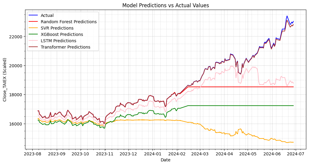
Random Forest MSE: 2539254.211486759
SVR MSE: 13866232.398817357
XGBoost MSE: 5859048.979625798
LSTM MSE: 1753263.4853189574
Transformer MSE: 2732.7598143748187
import os
import pandas as pd
import numpy as np
import matplotlib.pyplot as plt
import matplotlib.dates as mdates
from sklearn.preprocessing import StandardScaler
from sklearn.ensemble import RandomForestRegressor
from sklearn.svm import SVR
import tensorflow as tf
from tensorflow.keras.models import Sequential
from tensorflow.keras.layers import LSTM, Dense, Dropout
from xgboost import XGBRegressor
from sklearn.metrics import mean_squared_error
from google.colab import drive

# 掛載Google Drive
drive.mount('/content/drive')

# 確認文件路徑
file_path = '/content/drive/My Drive/MSCI_Taiwan_30_data_with_OBV.csv'
if os.path.exists(file_path):
    print("File exists")
    data = pd.read_csv(file_path)
else:
    print("File does not exist")

# 打印列名以檢查是否包含'Close'列
print(data.columns)

# 將'Close_MSCI'改為'Close'
if 'Close_MSCI' in data.columns:
    data.rename(columns={'Close_MSCI': 'Close'}, inplace=True)

# 確保日期列已經轉換為 datetime 類型
data['Date'] = pd.to_datetime(data['Date'])

# 計算移動平均線 (SMA)
if 'Close' in data.columns:
    data['MA10'] = data['Close'].rolling(window=10).mean()
    data['MA50'] = data['Close'].rolling(window=50).mean()
else:
    print("The 'Close' column is not found in the data.")
    raise KeyError("The 'Close' column is not found in the data.")

# 計算相對強弱指數 (RSI)
def compute_rsi(data, window=14):
    delta = data['Close'].diff(1)
    gain = (delta.where(delta > 0, 0)).rolling(window=window).mean()
    loss = (-delta.where(delta < 0, 0)).rolling(window=window).mean()
    rs = gain / loss
    rsi = 100 - (100 / (1 + rs))
    return rsi

data['RSI'] = compute_rsi(data)

# 計算移動平均收斂背離 (MACD)
def compute_macd(data, fast=12, slow=26, signal=9):
    exp1 = data['Close'].ewm(span=fast, adjust=False).mean()
    exp2 = data['Close'].ewm(span=slow, adjust=False).mean()
    macd = exp1 - exp2
    signal_line = macd.ewm(span=signal, adjust=False).mean()
    macd_hist = macd - signal_line
    return macd, signal_line, macd_hist

data['MACD'], data['MACD_Signal'], data['MACD_Hist'] = compute_macd(data)

# 填補缺失值
numeric_columns = data.select_dtypes(include=[np.number]).columns
data[numeric_columns] = data[numeric_columns].fillna(data[numeric_columns].mean())

# 選擇數值列進行相關性分析
numeric_data = data.select_dtypes(include=[np.number])

# 特徵選擇
correlation_matrix = numeric_data.corr()
target_corr = correlation_matrix['Close_TAIEX'].abs().sort_values(ascending=False)
selected_features = target_corr[target_corr > 0.5].index

# 特徵縮放
scaled_data = StandardScaler().fit_transform(numeric_data[selected_features])
scaled_data = pd.DataFrame(scaled_data, columns=selected_features)

# 分割數據為訓練集和測試集
train_size = int(len(data) * 0.8)
train_data = scaled_data[:train_size]
test_data = scaled_data[train_size:]

train_labels = data['Close_TAIEX'][:train_size]
test_labels = data['Close_TAIEX'][train_size:]

# 檢查數據長度
print(f"Train data length: {len(train_data)}")
print(f"Test data length: {len(test_data)}")
print(f"Train labels length: {len(train_labels)}")
print(f"Test labels length: {len(test_labels)}")

# 訓練隨機森林模型
rf_model = RandomForestRegressor(n_estimators=10, max_depth=None, min_samples_split=2, min_samples_leaf=1, max_features='auto')
rf_model.fit(train_data, train_labels)
rf_predictions = rf_model.predict(test_data)

# 訓練支持向量回歸模型 (SVR)
svr_model = SVR(C=1.0, epsilon=0.1, kernel='rbf', gamma='scale')
svr_model.fit(train_data, train_labels)
svr_predictions = svr_model.predict(test_data)

# 訓練XGBoost模型
xgb_model = XGBRegressor(n_estimators=10, max_depth=6, learning_rate=0.1, subsample=1.0)
xgb_model.fit(train_data, train_labels)
xgb_predictions = xgb_model.predict(test_data)

# 訓練改進後的LSTM模型
lstm_model = Sequential()
lstm_model.add(LSTM(10, return_sequences=True, input_shape=(train_data.shape[1], 1)))
lstm_model.add(Dropout(0.2))
lstm_model.add(LSTM(10, return_sequences=True))
lstm_model.add(Dropout(0.2))
lstm_model.add(LSTM(10, return_sequences=False))
lstm_model.add(Dropout(0.2))
lstm_model.add(Dense(10))
lstm_model.add(Dense(1))

lstm_model.compile(optimizer='adam', loss='mean_squared_error')
lstm_model.fit(np.expand_dims(train_data, axis=2), train_labels, batch_size=32, epochs=50)  # 增加訓練週期數
lstm_predictions = lstm_model.predict(np.expand_dims(test_data, axis=2))

# 訓練Transformer模型
class TransformerTimeSeries(tf.keras.Model):
    def __init__(self, num_layers, d_model, num_heads, dff, target_size, max_seq_len, rate=0.1):
        super(TransformerTimeSeries, self).__init__()
        self.encoder = tf.keras.layers.Dense(d_model)
        self.pos_encoding = self.positional_encoding(max_seq_len, d_model)
        self.transformer_blocks = [tf.keras.layers.MultiHeadAttention(num_heads, d_model) for _ in range(num_layers)]
        self.dense = tf.keras.layers.Dense(target_size)

    def positional_encoding(self, position, d_model):
        angle_rads = self.get_angles(np.arange(position)[:, np.newaxis], np.arange(d_model)[np.newaxis, :], d_model)
        sines = np.sin(angle_rads[:, 0::2])
        cosines = np.cos(angle_rads[:, 1::2])
        pos_encoding = np.concatenate([sines, cosines], axis=-1)
        pos_encoding = pos_encoding[np.newaxis, ...]
        return tf.cast(pos_encoding, dtype=tf.float32)

    def get_angles(self, pos, i, d_model):
        angle_rates = 1 / np.power(10000, (2 * (i // 2)) / np.float32(d_model))
        return pos * angle_rates

    def call(self, x):
        seq_len = tf.shape(x)[1]
        x = self.encoder(x)
        x += self.pos_encoding[:, :seq_len, :]
        for transformer_block in self.transformer_blocks:
            x = transformer_block(x, x)
        return self.dense(x)

transformer_model = TransformerTimeSeries(num_layers=1, d_model=16, num_heads=2, dff=32, target_size=1, max_seq_len=train_data.shape[1])
transformer_model.compile(optimizer='adam', loss='mean_squared_error')
transformer_model.fit(np.expand_dims(train_data, axis=2), train_labels, batch_size=32, epochs=50)  # 增加訓練週期數
transformer_predictions = transformer_model.predict(np.expand_dims(test_data, axis=2))

# 將transformer_predictions從3維轉為2維
transformer_predictions = np.squeeze(transformer_predictions)

# 調試信息
print("Shapes:")
print(f"test_labels: {test_labels.shape}")
print(f"transformer_predictions: {transformer_predictions.shape}")

# 確保transformer_predictions和test_labels形狀匹配
if transformer_predictions.ndim > 1:
    transformer_predictions = transformer_predictions[:, 0]

# 檢查調整後的形狀
print(f"Adjusted transformer_predictions shape: {transformer_predictions.shape}")

# 計算並打印各模型的MSE
print(f"Random Forest MSE: {mean_squared_error(test_labels, rf_predictions)}")
print(f"SVR MSE: {mean_squared_error(test_labels, svr_predictions)}")
print(f"XGBoost MSE: {mean_squared_error(test_labels, xgb_predictions)}")
print(f"LSTM MSE: {mean_squared_error(test_labels, lstm_predictions)}")
print(f"Transformer MSE: {mean_squared_error(test_labels, transformer_predictions)}")

# 繪製實際值與預測值的圖表
plt.figure(figsize=(12, 6))

# 繪製實際值
plt.plot(data['Date'][train_size:], test_labels, label='Actual', color='blue', linewidth=1.5)

# 繪製隨機森林預測值
plt.plot(data['Date'][train_size:], rf_predictions, label='Random Forest Predictions', color='red', linewidth=1.5)

# 繪製SVR預測值
plt.plot(data['Date'][train_size:], svr_predictions, label='SVR Predictions', color='orange', linewidth=1.5)

# 繪製XGBoost預測值
plt.plot(data['Date'][train_size:], xgb_predictions, label='XGBoost Predictions', color='green', linewidth=1.5)

# 繪製LSTM預測值
plt.plot(data['Date'][train_size:], lstm_predictions, label='LSTM Predictions', color='pink', linewidth=1.5)

# 繪製Transformer預測值
plt.plot(data['Date'][train_size:], transformer_predictions, label='Transformer Predictions', color='brown', linewidth=1.5)

plt.title('Model Predictions vs Actual Values')
plt.xlabel('Date')
plt.ylabel('Close_TAIEX (Scaled)')
plt.legend()

# 設置日期格式和標注每月的第一天
plt.gca().xaxis.set_major_locator(mdates.MonthLocator())
plt.gca().xaxis.set_major_formatter(mdates.DateFormatter('%Y-%m'))

# 添加網格
plt.grid(True, which='both', linestyle='--', linewidth=0.5)
plt.minorticks_on()
plt.grid(True, which='minor', linestyle=':', linewidth=0.5)

# 顯示圖表
plt.show()
隨機森林模型(Random Forest Regressor)
- 模型:
RandomForestRegressor - 參數:
n_estimators: 10(樹的數量)max_depth: None(樹的最大深度)min_samples_split: 2(內部節點再劃分所需的最小樣本數)min_samples_leaf: 1(葉子節點所需的最小樣本數)max_features: 'auto'(每次分裂時考慮的最大特徵數)
支持向量回歸模型(Support Vector Regressor, SVR)
- 模型:
SVR - 參數:
C: 1.0(懲罰係數)epsilon: 0.1(損失函數中沒有懲罰的間隔帶寬度)kernel: 'rbf'(核函數類型,徑向基函數)gamma: 'scale'(核係數)
XGBoost 模型(XGBoost Regressor)
- 模型:
XGBRegressor - 參數:
n_estimators: 10(樹的數量)max_depth: 6(樹的最大深度)learning_rate: 0.1(學習率)subsample: 1.0(訓練每棵樹時使用的樣本比例)
LSTM 模型(Long Short-Term Memory)
- 模型:
Sequential - 層:
- 第一層 LSTM: 10 個單元,
return_sequences=True,輸入形狀(train_data.shape[1], 1) - Dropout: 0.2
- 第二層 LSTM: 10 個單元,
return_sequences=True - Dropout: 0.2
- 第三層 LSTM: 10 個單元,
return_sequences=False - Dropout: 0.2
- Dense: 10 個單元
- Dense: 1 個單元
- 第一層 LSTM: 10 個單元,
- 訓練參數:
- 優化器:
adam - 損失函數:
mean_squared_error - 批量大小: 32
- 訓練周期數(epochs): 50
- 優化器:
Transformer 模型
- 模型: 自定義的
TransformerTimeSeries - 參數:
num_layers: 1(Transformer 層數)d_model: 16(嵌入維度)num_heads: 2(注意力頭數)dff: 32(前饋網絡的隱藏層大小)target_size: 1(輸出尺寸)max_seq_len:train_data.shape[1](序列最大長度)rate: 0.1(Dropout 率)
- 訓練參數:
- 優化器:
adam - 損失函數:
mean_squared_error - 批量大小: 32
- 訓練周期數(epochs): 50
- 優化器: