**TAIEX.s43_Training.3th.RandomForest+SVR+XGB+Transformer. 訓練4

Picture 1

Shapes:
test_labels: (6540,)
transformer_predictions: (6540, 2)
Adjusted transformer_predictions shape: (6540,)
Random Forest MSE: 2538928.7593811294
SVR MSE: 13866232.38063333
XGBoost MSE: 5859048.980611635
LSTM MSE: 1862506.720476739
Transformer MSE: 0.020672246942703427

import os
import pandas as pd
import numpy as np
import matplotlib.pyplot as plt
import matplotlib.dates as mdates
from sklearn.preprocessing import StandardScaler
from sklearn.ensemble import RandomForestRegressor
from sklearn.svm import SVR
import tensorflow as tf
from tensorflow.keras.models import Sequential
from tensorflow.keras.layers import LSTM, Dense, Dropout
from xgboost import XGBRegressor
from sklearn.metrics import mean_squared_error
from google.colab import drive

# 掛載Google Drive
drive.mount('/content/drive')

# 確認文件路徑
file_path = '/content/drive/My Drive/MSCI_Taiwan_30_data_with_OBV.csv'
if os.path.exists(file_path):
    print("File exists")
    data = pd.read_csv(file_path)
else:
    print("File does not exist")

# 打印列名以檢查是否包含'Close'列
print(data.columns)

# 將'Close_MSCI'改為'Close'
if 'Close_MSCI' in data.columns:
    data.rename(columns={'Close_MSCI': 'Close'}, inplace=True)

# 確保日期列已經轉換為 datetime 類型
data['Date'] = pd.to_datetime(data['Date'])

# 計算移動平均線 (SMA)
if 'Close' in data.columns:
    data['MA10'] = data['Close'].rolling(window=10).mean()
    data['MA50'] = data['Close'].rolling(window=50).mean()
else:
    print("The 'Close' column is not found in the data.")
    raise KeyError("The 'Close' column is not found in the data.")

# 計算相對強弱指數 (RSI)
def compute_rsi(data, window=14):
    delta = data['Close'].diff(1)
    gain = (delta.where(delta > 0, 0)).rolling(window=window).mean()
    loss = (-delta.where(delta < 0, 0)).rolling(window=window).mean()
    rs = gain / loss
    rsi = 100 - (100 / (1 + rs))
    return rsi

data['RSI'] = compute_rsi(data)

# 計算移動平均收斂背離 (MACD)
def compute_macd(data, fast=12, slow=26, signal=9):
    exp1 = data['Close'].ewm(span=fast, adjust=False).mean()
    exp2 = data['Close'].ewm(span=slow, adjust=False).mean()
    macd = exp1 - exp2
    signal_line = macd.ewm(span=signal, adjust=False).mean()
    macd_hist = macd - signal_line
    return macd, signal_line, macd_hist

data['MACD'], data['MACD_Signal'], data['MACD_Hist'] = compute_macd(data)

# 填補缺失值
numeric_columns = data.select_dtypes(include=[np.number]).columns
data[numeric_columns] = data[numeric_columns].fillna(data[numeric_columns].mean())

# 選擇數值列進行相關性分析
numeric_data = data.select_dtypes(include=[np.number])

# 特徵選擇
correlation_matrix = numeric_data.corr()
target_corr = correlation_matrix['Close_TAIEX'].abs().sort_values(ascending=False)
selected_features = target_corr[target_corr > 0.5].index

# 特徵縮放
scaled_data = StandardScaler().fit_transform(numeric_data[selected_features])
scaled_data = pd.DataFrame(scaled_data, columns=selected_features)

# 分割數據為訓練集和測試集
train_size = int(len(data) * 0.8)
train_data = scaled_data[:train_size]
test_data = scaled_data[train_size:]

train_labels = data['Close_TAIEX'][:train_size]
test_labels = data['Close_TAIEX'][train_size:]

# 檢查數據長度
print(f"Train data length: {len(train_data)}")
print(f"Test data length: {len(test_data)}")
print(f"Train labels length: {len(train_labels)}")
print(f"Test labels length: {len(test_labels)}")

# 訓練隨機森林模型
rf_model = RandomForestRegressor(n_estimators=10, max_depth=None, min_samples_split=2, min_samples_leaf=1, max_features='auto')
rf_model.fit(train_data, train_labels)
rf_predictions = rf_model.predict(test_data)

# 訓練支持向量回歸模型 (SVR)
svr_model = SVR(C=1.0, epsilon=0.1, kernel='rbf', gamma='scale')
svr_model.fit(train_data, train_labels)
svr_predictions = svr_model.predict(test_data)

# 訓練XGBoost模型
xgb_model = XGBRegressor(n_estimators=10, max_depth=6, learning_rate=0.1, subsample=1.0)
xgb_model.fit(train_data, train_labels)
xgb_predictions = xgb_model.predict(test_data)

# 訓練改進後的LSTM模型
lstm_model = Sequential()
lstm_model.add(LSTM(10, return_sequences=True, input_shape=(train_data.shape[1], 1)))
lstm_model.add(Dropout(0.2))
lstm_model.add(LSTM(10, return_sequences=True))
lstm_model.add(Dropout(0.2))
lstm_model.add(LSTM(10, return_sequences=False))
lstm_model.add(Dropout(0.2))
lstm_model.add(Dense(10))
lstm_model.add(Dense(1))

lstm_model.compile(optimizer='adam', loss='mean_squared_error')
lstm_model.fit(np.expand_dims(train_data, axis=2), train_labels, batch_size=32, epochs=50)  # 增加訓練週期數
lstm_predictions = lstm_model.predict(np.expand_dims(test_data, axis=2))

# 訓練Transformer模型
class TransformerTimeSeries(tf.keras.Model):
    def __init__(self, num_layers, d_model, num_heads, dff, target_size, max_seq_len, rate=0.1):
        super(TransformerTimeSeries, self).__init__()
        self.encoder = tf.keras.layers.Dense(d_model)
        self.pos_encoding = self.positional_encoding(max_seq_len, d_model)
        self.transformer_blocks = [tf.keras.layers.MultiHeadAttention(num_heads, d_model) for _ in range(num_layers)]
        self.dense = tf.keras.layers.Dense(target_size)

    def positional_encoding(self, position, d_model):
        angle_rads = self.get_angles(np.arange(position)[:, np.newaxis], np.arange(d_model)[np.newaxis, :], d_model)
        sines = np.sin(angle_rads[:, 0::2])
        cosines = np.cos(angle_rads[:, 1::2])
        pos_encoding = np.concatenate([sines, cosines], axis=-1)
        pos_encoding = pos_encoding[np.newaxis, ...]
        return tf.cast(pos_encoding, dtype=tf.float32)

    def get_angles(self, pos, i, d_model):
        angle_rates = 1 / np.power(10000, (2 * (i // 2)) / np.float32(d_model))
        return pos * angle_rates

    def call(self, x):
        seq_len = tf.shape(x)[1]
        x = self.encoder(x)
        x += self.pos_encoding[:, :seq_len, :]
        for transformer_block in self.transformer_blocks:
            x = transformer_block(x, x)
        return self.dense(x)

transformer_model = TransformerTimeSeries(num_layers=1, d_model=16, num_heads=2, dff=32, target_size=1, max_seq_len=train_data.shape[1])
transformer_model.compile(optimizer='adam', loss='mean_squared_error')
transformer_model.fit(np.expand_dims(train_data, axis=2), train_labels, batch_size=32, epochs=50)  # 增加訓練週期數
transformer_predictions = transformer_model.predict(np.expand_dims(test_data, axis=2))

# 將transformer_predictions從3維轉為2維
transformer_predictions = np.squeeze(transformer_predictions)

# 調試信息
print("Shapes:")
print(f"test_labels: {test_labels.shape}")
print(f"transformer_predictions: {transformer_predictions.shape}")

# 確保transformer_predictions和test_labels形狀匹配
if transformer_predictions.ndim > 1:
    transformer_predictions = transformer_predictions[:, 0]

# 檢查調整後的形狀
print(f"Adjusted transformer_predictions shape: {transformer_predictions.shape}")

# 計算並打印各模型的MSE
print(f"Random Forest MSE: {mean_squared_error(test_labels, rf_predictions)}")
print(f"SVR MSE: {mean_squared_error(test_labels, svr_predictions)}")
print(f"XGBoost MSE: {mean_squared_error(test_labels, xgb_predictions)}")
print(f"LSTM MSE: {mean_squared_error(test_labels, lstm_predictions)}")
print(f"Transformer MSE: {mean_squared_error(test_labels, transformer_predictions)}")

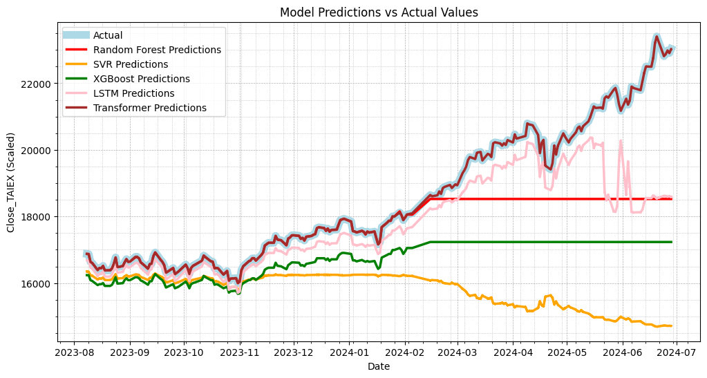
# 繪製實際值與預測值的圖表
plt.figure(figsize=(12, 6))

# 繪製實際值
plt.plot(data['Date'][train_size:], test_labels, label='Actual', color='blue', linewidth=5)

# 繪製隨機森林預測值
plt.plot(data['Date'][train_size:], rf_predictions, label='Random Forest Predictions', color='red', linewidth=2.5)

# 繪製SVR預測值
plt.plot(data['Date'][train_size:], svr_predictions, label='SVR Predictions', color='orange', linewidth=2.5)

# 繪製XGBoost預測值
plt.plot(data['Date'][train_size:], xgb_predictions, label='XGBoost Predictions', color='green', linewidth=2.5)

# 繪製LSTM預測值
plt.plot(data['Date'][train_size:], lstm_predictions, label='LSTM Predictions', color='pink', linewidth=2.5)

# 繪製Transformer預測值
plt.plot(data['Date'][train_size:], transformer_predictions, label='Transformer Predictions', color='brown', linewidth=2.5)

plt.title('Model Predictions vs Actual Values')
plt.xlabel('Date')
plt.ylabel('Close_TAIEX (Scaled)')
plt.legend()

# 設置日期格式和標注每月的第一天
plt.gca().xaxis.set_major_locator(mdates.MonthLocator())
plt.gca().xaxis.set_major_formatter(mdates.DateFormatter('%Y-%m'))

# 添加網格
plt.grid(True, which='both', linestyle='--', linewidth=0.5)
plt.minorticks_on()
plt.grid(True, which='minor', linestyle=':', linewidth=0.5)

# 顯示圖表
plt.show()

print("Selected features:", selected_features)

Picture 2

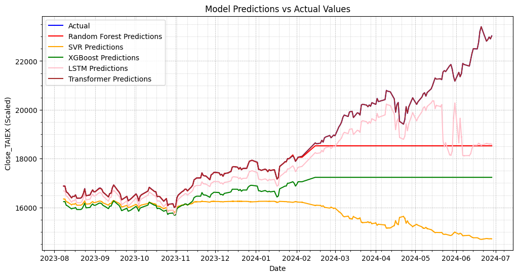
# 繪製實際值與預測值的圖表
plt.figure(figsize=(12, 6))

# 繪製實際值
plt.plot(data['Date'][train_size:], test_labels, label='Actual', color='lightblue', linewidth=8)

# 繪製隨機森林預測值
plt.plot(data['Date'][train_size:], rf_predictions, label='Random Forest Predictions', color='red', linewidth=2.5)

# 繪製SVR預測值
plt.plot(data['Date'][train_size:], svr_predictions, label='SVR Predictions', color='orange', linewidth=2.5)

# 繪製XGBoost預測值
plt.plot(data['Date'][train_size:], xgb_predictions, label='XGBoost Predictions', color='green', linewidth=2.5)

# 繪製LSTM預測值
plt.plot(data['Date'][train_size:], lstm_predictions, label='LSTM Predictions', color='pink', linewidth=2.5)

# 繪製Transformer預測值
plt.plot(data['Date'][train_size:], transformer_predictions, label='Transformer Predictions', color='brown', linewidth=2.5)

plt.title('Model Predictions vs Actual Values')
plt.xlabel('Date')
plt.ylabel('Close_TAIEX (Scaled)')
plt.legend()

# 設置日期格式和標注每月的第一天
plt.gca().xaxis.set_major_locator(mdates.MonthLocator())
plt.gca().xaxis.set_major_formatter(mdates.DateFormatter('%Y-%m'))

# 添加網格
plt.grid(True, which='both', linestyle='--', linewidth=0.5)
plt.minorticks_on()
plt.grid(True, which='minor', linestyle=':', linewidth=0.5)

# 顯示圖表
plt.show()

print("Selected features:", selected_features)