Predict

TAIEX.s91_練習使用 RandomForest 選擇特徵值的用法 + RFE 試作

cy.lu

03 Jul 2024 • 10 min read

Output

Shapes:
test_labels: (6540,)
transformer_predictions: (6540, 10)
Adjusted transformer_predictions shape: (6540,)
Random Forest MSE: 2545495.9702350823
SVR MSE: 9719829.364170404
XGBoost MSE: 2829341.20223588
LSTM MSE: 346273600.6513799
Transformer MSE: 16777426.64694445
Random Forest MAE: 903.3660629908254
SVR MAE: 2474.4028472217
XGBoost MAE: 999.7728105920297
LSTM MAE: 18499.252582865804
Transformer MAE: 3072.4997721785167

Selected features: Index(['Close_TAIEX', 'Market Return', 'OBV', 'RSI7', 'RSI21', 'RSI14','Aroon Down', '%K', 'CCI20', '%D'],dtype='object')

use Random Forest for feature selection

# Fill missing values
numeric_columns = data.select_dtypes(include=[np.number]).columns
data[numeric_columns] = data[numeric_columns].fillna(data[numeric_columns].mean())

# Select numeric columns for correlation analysis
numeric_data = data.select_dtypes(include=[np.number])

# Feature scaling
scaler = StandardScaler()
scaled_data = scaler.fit_transform(numeric_data)
scaled_data = pd.DataFrame(scaled_data, columns=numeric_columns)

# Split data into training and testing sets
train_size = int(len(data) * 0.8)
train_data = scaled_data[:train_size]
test_data = scaled_data[train_size:]

train_labels = data['Close_TAIEX'][:train_size]
test_labels = data['Close_TAIEX'][train_size:]

# Use Random Forest for feature selection
rf_selector = RandomForestRegressor(n_estimators=10)
rf_selector.fit(train_data, train_labels)

# Get feature importances and select top 10 features
feature_importances = pd.Series(rf_selector.feature_importances_, index=train_data.columns)
selected_features = feature_importances.nlargest(10).index

# Use only selected features
train_data = train_data[selected_features]
test_data = test_data[selected_features]

Source Code

import os
import pandas as pd
import numpy as np
import matplotlib.pyplot as plt
import matplotlib.dates as mdates
from sklearn.preprocessing import StandardScaler
from sklearn.ensemble import RandomForestRegressor
from sklearn.svm import SVR
import tensorflow as tf
from tensorflow.keras.models import Sequential
from tensorflow.keras.layers import LSTM, Dense, Dropout
from xgboost import XGBRegressor
from sklearn.metrics import mean_squared_error, mean_absolute_error
from google.colab import drive

# Mount Google Drive
drive.mount('/content/drive')

# Check file path
file_path = '/content/drive/My Drive/MSCI_Taiwan_30_data_with_OBV.csv'
if os.path.exists(file_path):
    print("File exists")
    data = pd.read_csv(file_path)
else:
    print("File does not exist")

# Print column names to check for 'Close' column
print(data.columns)

# Ensure 'Date' column is in datetime format
data['Date'] = pd.to_datetime(data['Date'])

# Fill missing values
numeric_columns = data.select_dtypes(include=[np.number]).columns
data[numeric_columns] = data[numeric_columns].fillna(data[numeric_columns].mean())

# Select numeric columns for correlation analysis
numeric_data = data.select_dtypes(include=[np.number])

# Feature scaling
scaler = StandardScaler()
scaled_data = scaler.fit_transform(numeric_data)
scaled_data = pd.DataFrame(scaled_data, columns=numeric_columns)

# Split data into training and testing sets
train_size = int(len(data) * 0.8)
train_data = scaled_data[:train_size]
test_data = scaled_data[train_size:]

train_labels = data['Close_TAIEX'][:train_size]
test_labels = data['Close_TAIEX'][train_size:]

# Use Random Forest for feature selection
rf_selector = RandomForestRegressor(n_estimators=10)
rf_selector.fit(train_data, train_labels)

# Get feature importances and select top 10 features
feature_importances = pd.Series(rf_selector.feature_importances_, index=train_data.columns)
selected_features = feature_importances.nlargest(10).index

# Use only selected features
train_data = train_data[selected_features]
test_data = test_data[selected_features]

# Check data lengths
print(f"Train data length: {len(train_data)}")
print(f"Test data length: {len(test_data)}")
print(f"Train labels length: {len(train_labels)}")
print(f"Test labels length: {len(test_labels)}")

# Train Random Forest model
rf_model = RandomForestRegressor(n_estimators=10)
rf_model.fit(train_data, train_labels)
rf_predictions = rf_model.predict(test_data)

# Train SVR model
svr_model = SVR(C=1.0, epsilon=0.1)
svr_model.fit(train_data, train_labels)
svr_predictions = svr_model.predict(test_data)

# Train XGBoost model
xgb_model = XGBRegressor(n_estimators=10)
xgb_model.fit(train_data, train_labels)
xgb_predictions = xgb_model.predict(test_data)

# Train LSTM model
lstm_model = Sequential()
lstm_model.add(LSTM(10, return_sequences=True, input_shape=(train_data.shape[1], 1)))
lstm_model.add(Dropout(0.2))
lstm_model.add(LSTM(10, return_sequences=False))
lstm_model.add(Dropout(0.2))
lstm_model.add(Dense(1))

lstm_model.compile(optimizer='adam', loss='mean_squared_error')
lstm_model.fit(np.expand_dims(train_data, axis=2), train_labels, epochs=5)  # Simplified training depth
lstm_predictions = lstm_model.predict(np.expand_dims(test_data, axis=2))

# Train Transformer model
class TransformerTimeSeries(tf.keras.Model):
    def __init__(self, num_layers, d_model, num_heads, dff, target_size, max_seq_len, rate=0.1):
        super(TransformerTimeSeries, self).__init__()
        self.encoder = tf.keras.layers.Dense(d_model)
        self.pos_encoding = self.positional_encoding(max_seq_len, d_model)
        self.transformer_blocks = [tf.keras.layers.MultiHeadAttention(num_heads, d_model) for _ in range(num_layers)]
        self.dense = tf.keras.layers.Dense(target_size)

    def positional_encoding(self, position, d_model):
        angle_rads = self.get_angles(np.arange(position)[:, np.newaxis], np.arange(d_model)[np.newaxis, :], d_model)
        sines = np.sin(angle_rads[:, 0::2])
        cosines = np.cos(angle_rads[:, 1::2])
        pos_encoding = np.concatenate([sines, cosines], axis=-1)
        pos_encoding = pos_encoding[np.newaxis, ...]
        return tf.cast(pos_encoding, dtype=tf.float32)

    def get_angles(self, pos, i, d_model):
        angle_rates = 1 / np.power(10000, (2 * (i // 2)) / np.float32(d_model))
        return pos * angle_rates

    def call(self, x):
        seq_len = tf.shape(x)[1]
        x = self.encoder(x)
        x += self.pos_encoding[:, :seq_len, :]
        for transformer_block in self.transformer_blocks:
            x = transformer_block(x, x)
        return self.dense(x)

transformer_model = TransformerTimeSeries(num_layers=1, d_model=16, num_heads=2, dff=32, target_size=1, max_seq_len=train_data.shape[1])
transformer_model.compile(optimizer='adam', loss='mean_squared_error')
transformer_model.fit(np.expand_dims(train_data, axis=2), train_labels, epochs=5)  # Simplified training depth
transformer_predictions = transformer_model.predict(np.expand_dims(test_data, axis=2))

# Transform transformer_predictions from 3D to 2D
transformer_predictions = np.squeeze(transformer_predictions)

# Debug information
print("Shapes:")
print(f"test_labels: {test_labels.shape}")
print(f"transformer_predictions: {transformer_predictions.shape}")

# Ensure transformer_predictions and test_labels shapes match
if transformer_predictions.ndim > 1:
    transformer_predictions = transformer_predictions[:, 0]

# Check adjusted shapes
print(f"Adjusted transformer_predictions shape: {transformer_predictions.shape}")

# Calculate and print MSE and MAE for each model
rf_mse = mean_squared_error(test_labels, rf_predictions)
svr_mse = mean_squared_error(test_labels, svr_predictions)
xgb_mse = mean_squared_error(test_labels, xgb_predictions)
lstm_mse = mean_squared_error(test_labels, lstm_predictions)
transformer_mse = mean_squared_error(test_labels, transformer_predictions)

rf_mae = mean_absolute_error(test_labels, rf_predictions)
svr_mae = mean_absolute_error(test_labels, svr_predictions)
xgb_mae = mean_absolute_error(test_labels, xgb_predictions)
lstm_mae = mean_absolute_error(test_labels, lstm_predictions)
transformer_mae = mean_absolute_error(test_labels, transformer_predictions)

print(f"Random Forest MSE: {rf_mse}")
print(f"SVR MSE: {svr_mse}")
print(f"XGBoost MSE: {xgb_mse}")
print(f"LSTM MSE: {lstm_mse}")
print(f"Transformer MSE: {transformer_mse}")

print(f"Random Forest MAE: {rf_mae}")
print(f"SVR MAE: {svr_mae}")
print(f"XGBoost MAE: {xgb_mae}")
print(f"LSTM MAE: {lstm_mae}")
print(f"Transformer MAE: {transformer_mae}")

# Plot actual values vs predictions
plt.figure(figsize=(12, 6))

# Plot actual values
plt.plot(data['Date'][train_size:], test_labels, label='Actual', color='lightblue', linewidth=8)

# Plot Random Forest predictions
plt.plot(data['Date'][train_size:], rf_predictions, label='Random Forest Predictions', color='red', linewidth=2.5)

# Plot SVR predictions
plt.plot(data['Date'][train_size:], svr_predictions, label='SVR Predictions', color='orange', linewidth=2.5)

# Plot XGBoost predictions
plt.plot(data['Date'][train_size:], xgb_predictions, label='XGBoost Predictions', color='green', linewidth=2.5)

# Plot LSTM predictions
plt.plot(data['Date'][train_size:], lstm_predictions, label='LSTM Predictions', color='pink', linewidth=2.5)

# Plot Transformer predictions
plt.plot(data['Date'][train_size:], transformer_predictions, label='Transformer Predictions', color='brown', linewidth=2.5)

plt.title('Model Predictions vs Actual Values')
plt.xlabel('Date')
plt.ylabel('Close_TAIEX (Scaled)')
plt.legend()

# Set date format and annotate the first day of each month
plt.gca().xaxis.set_major_locator(mdates.MonthLocator())
plt.gca().xaxis.set_major_formatter(mdates.DateFormatter('%Y-%m'))

# Set Y-axis limits
plt.ylim(13000, 26000)

# Add grid
plt.grid(True, which='both', linestyle='--', linewidth=0.5)
plt.minorticks_on()
plt.grid(True, which='minor', linestyle=':', linewidth=0.5)

# Show plot
plt.show()

print("Selected features:", selected_features)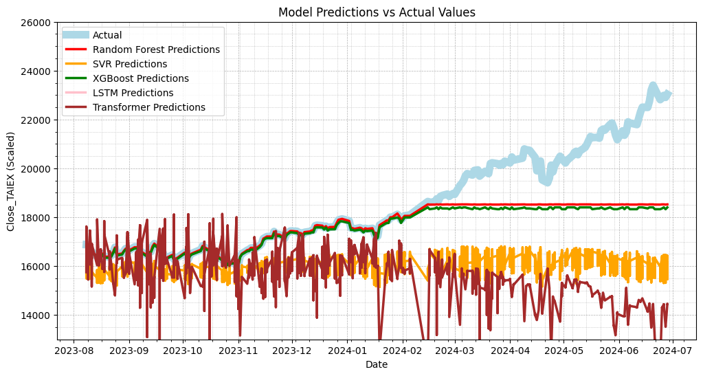

RFE

RFE（Recursive Feature Elimination，遞歸特徵消除）是一種特徵選擇技術，用於從初始特徵集中選擇最具影響力的特徵。其主要原理是通過遞歸地訓練模型、評估模型性能、移除對模型影響最小的特徵，從而找到最佳的特徵子集。以下是RFE的具體步驟：

初始化模型：
- 首先，選擇一個基礎模型，例如線性回歸、決策樹、支持向量機等。該模型將用於評估特徵的重要性。
訓練模型：
- 使用所有特徵訓練模型，並計算每個特徵的權重或重要性。
評估特徵：
- 根據模型的權重或重要性評估特徵。特徵的重要性可以通過模型係數、特徵得分等指標來衡量。
移除特徵：
- 移除對模型影響最小的特徵，即權重或得分最低的特徵。通常每次移除一個或一組特徵。
重複步驟2-4：
- 反復進行訓練模型、評估特徵和移除特徵的過程，直到達到預定的特徵數量或模型性能不再顯著提升。
選擇最佳特徵子集：
- 最終，選擇剩餘的特徵作為最佳特徵子集，這些特徵對模型性能影響最大。

RFE的優點

提高模型性能：通過消除不重要的特徵，可以減少模型的過擬合，從而提升模型的泛化能力和性能。
減少計算成本：選擇少量的重要特徵可以降低訓練和預測過程中的計算成本，特別是對於大規模數據集。
解釋性強：RFE選出的特徵往往對模型的解釋性更強，有助於理解特徵與目標變量之間的關係。


# Use RFE for feature selectionestimator = RandomForestRegressor(n_estimators=10)selector = RFE(estimator, n_features_to_select=10, step=1)selector = selector.fit(train_data, train_labels)selected_features = train_data.columns[selector.support_]
# Use only selected featurestrain_data = train_data[selected_features]test_data = test_data[selected_features]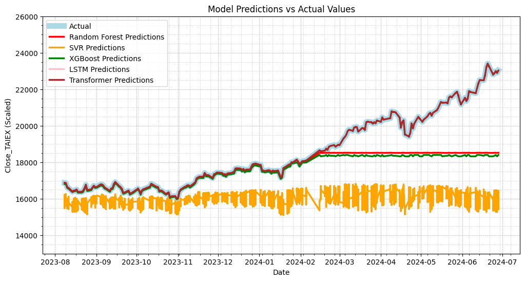

File exists
Index(['Date', 'ST_Code', 'ST_Name', 'Open', 'High', 'Low', 'Close',
       'Adj_Close', 'Volume', 'MA7', 'MA21', 'MA50', 'MA100', 'Middle Band',
       'Upper Band', 'Lower Band', 'Band Width', 'Aroon Up', 'Aroon Down',
       'CCI20', 'CMO14', 'MACD Line', 'Signal Line', 'MACD Histogram', 'RSI7',
       'RSI14', 'RSI21', '%K', '%D', 'WILLR14', 'Market Return',
       'Stock Return', 'Beta_60', 'Beta_120', 'Close_TAIEX', 'OBV'],
      dtype='object')
Train data length: 26160
Test data length: 6540
Train labels length: 26160
Test labels length: 6540


Shapes:
test_labels: (6540,)
transformer_predictions: (6540, 10)
Adjusted transformer_predictions shape: (6540,)
Random Forest MSE: 2545214.32235445
SVR MSE: 9710076.158648852
XGBoost MSE: 2829341.20223588
LSTM MSE: 346253938.61952394
Transformer MSE: 6.337947021220456
Random Forest MAE: 903.3790180229354
SVR MAE: 2472.872082309311
XGBoost MAE: 999.7728105920297
LSTM MAE: 18498.721145602663
Transformer MAE: 1.885159940319162

import os
import pandas as pd
import numpy as np
import matplotlib.pyplot as plt
import matplotlib.dates as mdates
from sklearn.preprocessing import StandardScaler
from sklearn.feature_selection import RFE
from sklearn.ensemble import RandomForestRegressor
from sklearn.svm import SVR
import tensorflow as tf
from tensorflow.keras.models import Sequential
from tensorflow.keras.layers import LSTM, Dense, Dropout
from xgboost import XGBRegressor
from sklearn.metrics import mean_squared_error, mean_absolute_error
from google.colab import drive

# Mount Google Drive
drive.mount('/content/drive')

# Check file path
file_path = '/content/drive/My Drive/MSCI_Taiwan_30_data_with_OBV.csv'
if os.path.exists(file_path):
    print("File exists")
    data = pd.read_csv(file_path)
else:
    print("File does not exist")

# Print column names to check for 'Close' column
print(data.columns)

# Ensure 'Date' column is in datetime format
data['Date'] = pd.to_datetime(data['Date'])

# Fill missing values
numeric_columns = data.select_dtypes(include=[np.number]).columns
data[numeric_columns] = data[numeric_columns].fillna(data[numeric_columns].mean())

# Select numeric columns for correlation analysis
numeric_data = data.select_dtypes(include=[np.number])

# Feature scaling
scaler = StandardScaler()
scaled_data = scaler.fit_transform(numeric_data)
scaled_data = pd.DataFrame(scaled_data, columns=numeric_columns)

# Split data into training and testing sets
train_size = int(len(data) * 0.8)
train_data = scaled_data[:train_size]
test_data = scaled_data[train_size:]

train_labels = data['Close_TAIEX'][:train_size]
test_labels = data['Close_TAIEX'][train_size:]

# Use RFE for feature selection
estimator = RandomForestRegressor(n_estimators=10)
selector = RFE(estimator, n_features_to_select=10, step=1)
selector = selector.fit(train_data, train_labels)
selected_features = train_data.columns[selector.support_]

# Use only selected features
train_data = train_data[selected_features]
test_data = test_data[selected_features]

# Check data lengths
print(f"Train data length: {len(train_data)}")
print(f"Test data length: {len(test_data)}")
print(f"Train labels length: {len(train_labels)}")
print(f"Test labels length: {len(test_labels)}")

# Train Random Forest model
rf_model = RandomForestRegressor(n_estimators=10)
rf_model.fit(train_data, train_labels)
rf_predictions = rf_model.predict(test_data)

# Train SVR model
svr_model = SVR(C=1.0, epsilon=0.1)
svr_model.fit(train_data, train_labels)
svr_predictions = svr_model.predict(test_data)

# Train XGBoost model
xgb_model = XGBRegressor(n_estimators=10)
xgb_model.fit(train_data, train_labels)
xgb_predictions = xgb_model.predict(test_data)

# Train LSTM model
lstm_model = Sequential()
lstm_model.add(LSTM(10, return_sequences=True, input_shape=(train_data.shape[1], 1)))
lstm_model.add(Dropout(0.2))
lstm_model.add(LSTM(10, return_sequences=False))
lstm_model.add(Dropout(0.2))
lstm_model.add(Dense(1))

lstm_model.compile(optimizer='adam', loss='mean_squared_error')
lstm_model.fit(np.expand_dims(train_data, axis=2), train_labels, epochs=5)  # Simplified training depth
lstm_predictions = lstm_model.predict(np.expand_dims(test_data, axis=2))

# Train Transformer model
class TransformerTimeSeries(tf.keras.Model):
    def __init__(self, num_layers, d_model, num_heads, dff, target_size, max_seq_len, rate=0.1):
        super(TransformerTimeSeries, self).__init__()
        self.encoder = tf.keras.layers.Dense(d_model)
        self.pos_encoding = self.positional_encoding(max_seq_len, d_model)
        self.transformer_blocks = [tf.keras.layers.MultiHeadAttention(num_heads, d_model) for _ in range(num_layers)]
        self.dense = tf.keras.layers.Dense(target_size)

    def positional_encoding(self, position, d_model):
        angle_rads = self.get_angles(np.arange(position)[:, np.newaxis], np.arange(d_model)[np.newaxis, :], d_model)
        sines = np.sin(angle_rads[:, 0::2])
        cosines = np.cos(angle_rads[:, 1::2])
        pos_encoding = np.concatenate([sines, cosines], axis=-1)
        pos_encoding = pos_encoding[np.newaxis, ...]
        return tf.cast(pos_encoding, dtype=tf.float32)

    def get_angles(self, pos, i, d_model):
        angle_rates = 1 / np.power(10000, (2 * (i // 2)) / np.float32(d_model))
        return pos * angle_rates

    def call(self, x):
        seq_len = tf.shape(x)[1]
        x = self.encoder(x)
        x += self.pos_encoding[:, :seq_len, :]
        for transformer_block in self.transformer_blocks:
            x = transformer_block(x, x)
        return self.dense(x)

transformer_model = TransformerTimeSeries(num_layers=1, d_model=16, num_heads=2, dff=32, target_size=1, max_seq_len=train_data.shape[1])
transformer_model.compile(optimizer='adam', loss='mean_squared_error')
transformer_model.fit(np.expand_dims(train_data, axis=2), train_labels, epochs=5)  # Simplified training depth
transformer_predictions = transformer_model.predict(np.expand_dims(test_data, axis=2))

# Transform transformer_predictions from 3D to 2D
transformer_predictions = np.squeeze(transformer_predictions)

# Debug information
print("Shapes:")
print(f"test_labels: {test_labels.shape}")
print(f"transformer_predictions: {transformer_predictions.shape}")

# Ensure transformer_predictions and test_labels shapes match
if transformer_predictions.ndim > 1:
    transformer_predictions = transformer_predictions[:, 0]

# Check adjusted shapes
print(f"Adjusted transformer_predictions shape: {transformer_predictions.shape}")

# Calculate and print MSE and MAE for each model
rf_mse = mean_squared_error(test_labels, rf_predictions)
svr_mse = mean_squared_error(test_labels, svr_predictions)
xgb_mse = mean_squared_error(test_labels, xgb_predictions)
lstm_mse = mean_squared_error(test_labels, lstm_predictions)
transformer_mse = mean_squared_error(test_labels, transformer_predictions)

rf_mae = mean_absolute_error(test_labels, rf_predictions)
svr_mae = mean_absolute_error(test_labels, svr_predictions)
xgb_mae = mean_absolute_error(test_labels, xgb_predictions)
lstm_mae = mean_absolute_error(test_labels, lstm_predictions)
transformer_mae = mean_absolute_error(test_labels, transformer_predictions)

print(f"Random Forest MSE: {rf_mse}")
print(f"SVR MSE: {svr_mse}")
print(f"XGBoost MSE: {xgb_mse}")
print(f"LSTM MSE: {lstm_mse}")
print(f"Transformer MSE: {transformer_mse}")

print(f"Random Forest MAE: {rf_mae}")
print(f"SVR MAE: {svr_mae}")
print(f"XGBoost MAE: {xgb_mae}")
print(f"LSTM MAE: {lstm_mae}")
print(f"Transformer MAE: {transformer_mae}")

# Plot actual values vs predictions
plt.figure(figsize=(12, 6))

# Plot actual values
plt.plot(data['Date'][train_size:], test_labels, label='Actual', color='lightblue', linewidth=8)

# Plot Random Forest predictions
plt.plot(data['Date'][train_size:], rf_predictions, label='Random Forest Predictions', color='red', linewidth=2.5)

# Plot SVR predictions
plt.plot(data['Date'][train_size:], svr_predictions, label='SVR Predictions', color='orange', linewidth=2.5)

# Plot XGBoost predictions
plt.plot(data['Date'][train_size:], xgb_predictions, label='XGBoost Predictions', color='green', linewidth=2.5)

# Plot LSTM predictions
plt.plot(data['Date'][train_size:], lstm_predictions, label='LSTM Predictions', color='pink', linewidth=2.5)

# Plot Transformer predictions
plt.plot(data['Date'][train_size:], transformer_predictions, label='Transformer Predictions', color='brown', linewidth=2.5)

plt.title('Model Predictions vs Actual Values')
plt.xlabel('Date')
plt.ylabel('Close_TAIEX (Scaled)')
plt.legend()

# Set date format and annotate the first day of each month
plt.gca().xaxis.set_major_locator(mdates.MonthLocator())
plt.gca().xaxis.set_major_formatter(mdates.DateFormatter('%Y-%m'))

# Set Y-axis limits
plt.ylim(13000, 26000)

# Add grid
plt.grid(True, which='both', linestyle='--', linewidth=0.5)
plt.minorticks_on()
plt.grid(True, which='minor', linestyle=':', linewidth=0.5)

# Show plot
plt.show()

print("Selected features:", selected_features)