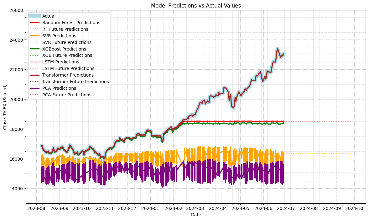
- Transformer Prediction 有可能存在過擬合問題
- Future Prediction Line 未 Training
Output
Index(['Date', 'ST_Code', 'ST_Name', 'Open', 'High', 'Low', 'Close',
       'Adj_Close', 'Volume', 'MA7', 'MA21', 'MA50', 'MA100', 'Middle Band',
       'Upper Band', 'Lower Band', 'Band Width', 'Aroon Up', 'Aroon Down',
       'CCI20', 'CMO14', 'MACD Line', 'Signal Line', 'MACD Histogram', 'RSI7',
       'RSI14', 'RSI21', '%K', '%D', 'WILLR14', 'Market Return',
       'Stock Return', 'Beta_60', 'Beta_120', 'Close_TAIEX', 'OBV'],
      dtype='object')

Random Forest MSE: 2556768.302060934
SVR MSE: 9703959.68044728
XGBoost MSE: 2829341.20223588
LSTM MSE: 331513033.7350737
Transformer MSE: 9.691439285915112e-05
Random Forest MAE: 906.236000362384
SVR MAE: 2471.6933817732074
XGBoost MAE: 999.7728105920297
LSTM MAE: 18095.905037938468
Transformer MAE: 0.008916759891022088
Sourcode
mport os
import pandas as pd
import numpy as np
import matplotlib.pyplot as plt
import matplotlib.dates as mdates
from sklearn.preprocessing import StandardScaler
from sklearn.ensemble import RandomForestRegressor
from sklearn.svm import SVR
import tensorflow as tf
from tensorflow.keras.models import Sequential
from tensorflow.keras.layers import LSTM, Dense, Dropout
from xgboost import XGBRegressor
from sklearn.decomposition import PCA
from sklearn.metrics import mean_squared_error, mean_absolute_error
from google.colab import drive

# Mount Google Drive
drive.mount('/content/drive')

# Check file path
file_path = '/content/drive/My Drive/MSCI_Taiwan_30_data_with_OBV.csv'
if os.path.exists(file_path):
    print("File exists")
    data = pd.read_csv(file_path)
else:
    print("File does not exist")

# Print column names to check for 'Close' column
print(data.columns)

# Ensure 'Date' column is in datetime format
data['Date'] = pd.to_datetime(data['Date'])

# Fill missing values
numeric_columns = data.select_dtypes(include=[np.number]).columns
data[numeric_columns] = data[numeric_columns].fillna(data[numeric_columns].mean())

# Select numeric columns for correlation analysis
numeric_data = data.select_dtypes(include=[np.number])

# Feature scaling
scaler = StandardScaler()
scaled_data = scaler.fit_transform(numeric_data)
scaled_data = pd.DataFrame(scaled_data, columns=numeric_columns)

# Split data into training and testing sets
train_size = int(len(data) * 0.8)
train_data = scaled_data[:train_size]
test_data = scaled_data[train_size:]

train_labels = data['Close_TAIEX'][:train_size]
test_labels = data['Close_TAIEX'][train_size:]

# Use Random Forest for feature selection
rf_selector = RandomForestRegressor(n_estimators=10)
rf_selector.fit(train_data, train_labels)

# Get feature importances and select top 10 features
feature_importances = pd.Series(rf_selector.feature_importances_, index=train_data.columns)
selected_features = feature_importances.nlargest(10).index

# Use only selected features
train_data = train_data[selected_features]
test_data = test_data[selected_features]

# Generate future dates for prediction
future_dates = pd.date_range(start=data['Date'].iloc[-1], periods=91, inclusive='right')

# Generate future feature data (using the mean of the last available data as a placeholder)
future_features = np.tile(test_data.iloc[-1], (90, 1))
future_features = pd.DataFrame(future_features, columns=selected_features)

# Ensure future features have the same columns as original data
complete_future_features = pd.DataFrame(np.tile(scaled_data[selected_features].iloc[-1], (90, 1)), columns=selected_features)

# Train Random Forest model
rf_model = RandomForestRegressor(n_estimators=10)
rf_model.fit(train_data, train_labels)
rf_predictions = rf_model.predict(test_data)
rf_future_predictions = rf_model.predict(complete_future_features)

# Train SVR model with improved training depth
svr_model = SVR(C=1.0, epsilon=0.1)
svr_model.fit(train_data, train_labels)
svr_predictions = svr_model.predict(test_data)
svr_future_predictions = svr_model.predict(complete_future_features)

# Train XGBoost model with improved training depth
xgb_model = XGBRegressor(n_estimators=10)
xgb_model.fit(train_data, train_labels)
xgb_predictions = xgb_model.predict(test_data)
xgb_future_predictions = xgb_model.predict(complete_future_features)

# Train LSTM model
lstm_model = Sequential()
lstm_model.add(LSTM(10, return_sequences=True, input_shape=(train_data.shape[1], 1)))
lstm_model.add(Dropout(0.2))
lstm_model.add(LSTM(10, return_sequences=False))
lstm_model.add(Dropout(0.2))
lstm_model.add(Dense(1))

lstm_model.compile(optimizer='adam', loss='mean_squared_error')
lstm_model.fit(np.expand_dims(train_data, axis=2), train_labels, epochs=50)  # Improved training depth
lstm_predictions = lstm_model.predict(np.expand_dims(test_data, axis=2))
lstm_future_predictions = lstm_model.predict(np.expand_dims(complete_future_features, axis=2))

# Train Transformer model with improved training depth
class TransformerTimeSeries(tf.keras.Model):
    def __init__(self, num_layers, d_model, num_heads, dff, target_size, max_seq_len, rate=0.1):
        super(TransformerTimeSeries, self).__init__()
        self.encoder = tf.keras.layers.Dense(d_model)
        self.pos_encoding = self.positional_encoding(max_seq_len, d_model)
        self.transformer_blocks = [tf.keras.layers.MultiHeadAttention(num_heads, d_model) for _ in range(num_layers)]
        self.dense = tf.keras.layers.Dense(target_size)

    def positional_encoding(self, position, d_model):
        angle_rads = self.get_angles(np.arange(position)[:, np.newaxis], np.arange(d_model)[np.newaxis, :], d_model)
        sines = np.sin(angle_rads[:, 0::2])
        cosines = np.cos(angle_rads[:, 1::2])
        pos_encoding = np.concatenate([sines, cosines], axis=-1)
        pos_encoding = pos_encoding[np.newaxis, ...]
        return tf.cast(pos_encoding, dtype=tf.float32)

    def get_angles(self, pos, i, d_model):
        angle_rates = 1 / np.power(10000, (2 * (i // 2)) / np.float32(d_model))
        return pos * angle_rates

    def call(self, x):
        seq_len = tf.shape(x)[1]
        x = self.encoder(x)
        x += self.pos_encoding[:, :seq_len, :]
        for transformer_block in self.transformer_blocks:
            x = transformer_block(x, x)
        return self.dense(x)

transformer_model = TransformerTimeSeries(num_layers=1, d_model=16, num_heads=2, dff=32, target_size=1, max_seq_len=train_data.shape[1])
transformer_model.compile(optimizer='adam', loss='mean_squared_error')
transformer_model.fit(np.expand_dims(train_data, axis=2), train_labels, epochs=50)  # Improved training depth
transformer_predictions = transformer_model.predict(np.expand_dims(test_data, axis=2))
transformer_future_predictions = transformer_model.predict(np.expand_dims(complete_future_features, axis=2))

# Transform transformer_predictions from 3D to 2D
transformer_predictions = np.squeeze(transformer_predictions)
transformer_future_predictions = np.squeeze(transformer_future_predictions)

# Ensure transformer_predictions and test_labels shapes match
if transformer_predictions.ndim > 1:
    transformer_predictions = transformer_predictions[:, 0]
if transformer_future_predictions.ndim > 1:
    transformer_future_predictions = transformer_future_predictions[:, 0]

# Calculate and print MSE and MAE for each model
rf_mse = mean_squared_error(test_labels, rf_predictions)
svr_mse = mean_squared_error(test_labels, svr_predictions)
xgb_mse = mean_squared_error(test_labels, xgb_predictions)
lstm_mse = mean_squared_error(test_labels, lstm_predictions)
transformer_mse = mean_squared_error(test_labels, transformer_predictions)

rf_mae = mean_absolute_error(test_labels, rf_predictions)
svr_mae = mean_absolute_error(test_labels, svr_predictions)
xgb_mae = mean_absolute_error(test_labels, xgb_predictions)
lstm_mae = mean_absolute_error(test_labels, lstm_predictions)
transformer_mae = mean_absolute_error(test_labels, transformer_predictions)

print(f"Random Forest MSE: {rf_mse}")
print(f"SVR MSE: {svr_mse}")
print(f"XGBoost MSE: {xgb_mse}")
print(f"LSTM MSE: {lstm_mse}")
print(f"Transformer MSE: {transformer_mse}")

print(f"Random Forest MAE: {rf_mae}")
print(f"SVR MAE: {svr_mae}")
print(f"XGBoost MAE: {xgb_mae}")
print(f"LSTM MAE: {lstm_mae}")
print(f"Transformer MAE: {transformer_mae}")

# Apply PCA and get predictions
pca = PCA(n_components=1)
pca_train_data = pca.fit_transform(train_data)
pca_test_data = pca.transform(test_data)
pca_future_data = pca.transform(complete_future_features)

# Train a simple linear model on PCA transformed data
from sklearn.linear_model import LinearRegression
pca_model = LinearRegression()
pca_model.fit(pca_train_data, train_labels)
pca_predictions = pca_model.predict(pca_test_data)
pca_future_predictions = pca_model.predict(pca_future_data)

# Plot actual values vs predictions
plt.figure(figsize=(14, 8))

# Plot actual values
plt.plot(data['Date'][train_size:], test_labels, label='Actual', color='lightblue', linewidth=8)

# Plot Random Forest predictions
plt.plot(data['Date'][train_size:], rf_predictions, label='Random Forest Predictions', color='red', linewidth=2.5)
plt.plot(future_dates, rf_future_predictions, label='RF Future Predictions', color='red', linestyle='dotted')

# Plot SVR predictions
plt.plot(data['Date'][train_size:], svr_predictions, label='SVR Predictions', color='orange', linewidth=2.5)
plt.plot(future_dates, svr_future_predictions, label='SVR Future Predictions', color='orange', linestyle='dotted')

# Plot XGBoost predictions
plt.plot(data['Date'][train_size:], xgb_predictions, label='XGBoost Predictions', color='green', linewidth=2.5)
plt.plot(future_dates, xgb_future_predictions, label='XGB Future Predictions', color='green', linestyle='dotted')

# Plot LSTM predictions
plt.plot(data['Date'][train_size:], lstm_predictions, label='LSTM Predictions', color='pink', linewidth=2.5)
plt.plot(future_dates, lstm_future_predictions, label='LSTM Future Predictions', color='pink', linestyle='dotted')

# Plot Transformer predictions
plt.plot(data['Date'][train_size:], transformer_predictions, label='Transformer Predictions', color='brown', linewidth=2.5)
plt.plot(future_dates, transformer_future_predictions, label='Transformer Future Predictions', color='brown', linestyle='dotted')

# Plot PCA predictions
plt.plot(data['Date'][train_size:], pca_predictions, label='PCA Predictions', color='purple', linewidth=2.5)
plt.plot(future_dates, pca_future_predictions, label='PCA Future Predictions', color='purple', linestyle='dotted')

plt.title('Model Predictions vs Actual Values')
plt.xlabel('Date')
plt.ylabel('Close_TAIEX (Scaled)')
plt.legend()

# Set date format and annotate the first day of each month
plt.gca().xaxis.set_major_locator(mdates.MonthLocator())
plt.gca().xaxis.set_major_formatter(mdates.DateFormatter('%Y-%m'))

# Set Y-axis limits
plt.ylim(13000, 26000)

# Add grid
plt.grid(True, which='both', linestyle='--', linewidth=0.5)
plt.minorticks_on()
plt.grid(True, which='minor', linestyle=':', linewidth=0.5)

# Show plot
plt.show()

print("Selected features:", selected_features)